![]()
9.1 Maximum Likelihood Estimation (MLE)#
The Core Idea#
Maximum Likelihood Estimation: Find the parameter value that maximizes the probability of observing the data we actually observed.
The Likelihood Function#
Definition#
Given data (x_1, x_2, \ldots, x_n) and a model with parameter θ, the likelihood function is:
For Independent Data#
If observations are independent and identically distributed (i.i.d.):
where (f(x \mid \theta)) is the probability (PMF) or density (PDF).
Log-Likelihood#
In practice, we work with log-likelihood (easier to maximize):
The MLE#
Maximum Likelihood Estimate (\hat{\theta}_{\text{MLE}}) is the value that maximizes (L(\theta)) or (\ell(\theta)):
Finding the MLE#
Write down the likelihood (L(\theta))
Take the log: (\ell(\theta) = \log L(\theta))
Take the derivative: (\frac{d\ell}{d\theta})
Set equal to zero and solve: (\frac{d\ell}{d\theta} = 0)
Verify it’s a maximum (check second derivative < 0)
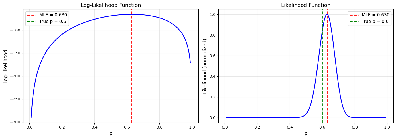
Example 1: Bernoulli Distribution#
Problem#
Flip a coin n times, observe k heads. Estimate p (probability of heads).
Solution#
Model: Each flip (X_i \sim \text{Bernoulli}(p))
Likelihood: $\( L(p) = \prod_{i=1}^{n} p^{x_i}(1-p)^{1-x_i} = p^k(1-p)^{n-k} \)$
where k = number of heads.
Log-likelihood: $\( \ell(p) = k\log p + (n-k)\log(1-p) \)$
Derivative: $\( \frac{d\ell}{dp} = \frac{k}{p} - \frac{n-k}{1-p} \)$
Set to zero: $\( \frac{k}{p} = \frac{n-k}{1-p} \implies k(1-p) = p(n-k) \implies k = np \)$
MLE: $\( \hat{p}_{\text{MLE}} = \frac{k}{n} \)$
The MLE is just the sample proportion!
Python Implementation#
import numpy as np
import matplotlib.pyplot as plt
from scipy import stats
from scipy.optimize import minimize_scalar

np.random.seed(42)

# Generate data: 100 flips with true p = 0.6
true_p = 0.6
n = 100
flips = np.random.binomial(1, true_p, n)
k = np.sum(flips)

print("Bernoulli MLE Example")
print("="*70)
print(f"True p: {true_p}")
print(f"Sample: {n} flips, {k} heads")
print()

# MLE
p_mle = k / n
print(f"MLE estimate: p̂ = {p_mle:.3f}")
print()

# Log-likelihood function
def log_likelihood_bernoulli(p, data):
    k = np.sum(data)
    n = len(data)
    if p <= 0 or p >= 1:
        return -np.inf
    return k * np.log(p) + (n - k) * np.log(1 - p)

# Plot likelihood function
p_values = np.linspace(0.01, 0.99, 1000)
log_likes = [log_likelihood_bernoulli(p, flips) for p in p_values]

fig, (ax1, ax2) = plt.subplots(1, 2, figsize=(14, 5))

# Log-likelihood
ax1.plot(p_values, log_likes, 'b-', linewidth=2)
ax1.axvline(p_mle, color='red', linestyle='--', linewidth=2,
            label=f'MLE = {p_mle:.3f}')
ax1.axvline(true_p, color='green', linestyle='--', linewidth=2,
            label=f'True p = {true_p}')
ax1.set_xlabel('p', fontsize=12)
ax1.set_ylabel('Log-Likelihood', fontsize=12)
ax1.set_title('Log-Likelihood Function', fontsize=13)
ax1.legend(fontsize=11)
ax1.grid(alpha=0.3)

# Likelihood (not log)
likes = np.exp(log_likes - np.max(log_likes))  # Normalize for plotting
ax2.plot(p_values, likes, 'b-', linewidth=2)
ax2.axvline(p_mle, color='red', linestyle='--', linewidth=2,
            label=f'MLE = {p_mle:.3f}')
ax2.axvline(true_p, color='green', linestyle='--', linewidth=2,
            label=f'True p = {true_p}')
ax2.set_xlabel('p', fontsize=12)
ax2.set_ylabel('Likelihood (normalized)', fontsize=12)
ax2.set_title('Likelihood Function', fontsize=13)
ax2.legend(fontsize=11)
ax2.grid(alpha=0.3)

plt.tight_layout()
plt.savefig('bernoulli_mle.png', dpi=150, bbox_inches='tight')
plt.show()
Bernoulli MLE Example
======================================================================
True p: 0.6
Sample: 100 flips, 63 heads

MLE estimate: p̂ = 0.630
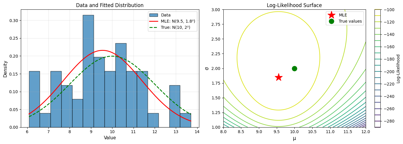
Example 2: Normal Distribution#
Problem#
Observe (x_1, \ldots, x_n \sim N(\mu, \sigma^2)). Estimate μ and σ².
Solution#
PDF: $\( f(x \mid \mu, \sigma^2) = \frac{1}{\sqrt{2\pi\sigma^2}}\exp\left(-\frac{(x-\mu)^2}{2\sigma^2}\right) \)$
Log-likelihood: $\( \ell(\mu, \sigma^2) = -\frac{n}{2}\log(2\pi) - \frac{n}{2}\log(\sigma^2) - \frac{1}{2\sigma^2}\sum_{i=1}^{n}(x_i - \mu)^2 \)$
Derivative w.r.t. μ: $\( \frac{\partial\ell}{\partial\mu} = \frac{1}{\sigma^2}\sum_{i=1}^{n}(x_i - \mu) = 0 \)$
MLE for μ: $\( \hat{\mu}_{\text{MLE}} = \frac{1}{n}\sum_{i=1}^{n}x_i = \bar{x} \)$
Derivative w.r.t. σ²: $\( \frac{\partial\ell}{\partial\sigma^2} = -\frac{n}{2\sigma^2} + \frac{1}{2(\sigma^2)^2}\sum_{i=1}^{n}(x_i - \mu)^2 = 0 \)$
MLE for σ²: $\( \hat{\sigma}^2_{\text{MLE}} = \frac{1}{n}\sum_{i=1}^{n}(x_i - \bar{x})^2 \)$
Note: This uses (n) in denominator, not (n-1) (slightly biased for small n).
Python Implementation#
import numpy as np
import matplotlib.pyplot as plt
from scipy import stats
from scipy.optimize import minimize

np.random.seed(42)

# Generate data
true_mu = 10
true_sigma = 2
n = 50
data = np.random.normal(true_mu, true_sigma, n)

print("Normal Distribution MLE")
print("="*70)
print(f"True μ: {true_mu}, True σ: {true_sigma}")
print(f"Sample size: {n}")
print()

# Analytical MLE
mu_mle = np.mean(data)
sigma2_mle = np.mean((data - mu_mle)**2)
sigma_mle = np.sqrt(sigma2_mle)

print("Analytical MLE:")
print(f"  μ̂ = {mu_mle:.3f}")
print(f"  σ̂ = {sigma_mle:.3f}")
print()

# Numerical MLE (for illustration)
def neg_log_likelihood_normal(params, data):
    mu, sigma = params
    if sigma <= 0:
        return np.inf
    n = len(data)
    return n/2 * np.log(2*np.pi) + n/2 * np.log(sigma**2) + \
           np.sum((data - mu)**2) / (2 * sigma**2)

# Optimize
initial_guess = [0, 1]
result = minimize(neg_log_likelihood_normal, initial_guess, args=(data,),
                  method='Nelder-Mead')

mu_mle_num, sigma_mle_num = result.x

print("Numerical MLE (verification):")
print(f"  μ̂ = {mu_mle_num:.3f}")
print(f"  σ̂ = {sigma_mle_num:.3f}")
print()

# Compare with true values
print("Comparison with true values:")
print(f"  μ: error = {abs(mu_mle - true_mu):.3f}")
print(f"  σ: error = {abs(sigma_mle - true_sigma):.3f}")

# Visualize
fig, (ax1, ax2) = plt.subplots(1, 2, figsize=(14, 5))

# Data histogram with fitted distribution
ax1.hist(data, bins=15, density=True, alpha=0.7, edgecolor='black',
         label='Data')
x = np.linspace(data.min(), data.max(), 100)
ax1.plot(x, stats.norm.pdf(x, mu_mle, sigma_mle), 'r-', linewidth=2,
         label=f'MLE: N({mu_mle:.1f}, {sigma_mle:.1f}²)')
ax1.plot(x, stats.norm.pdf(x, true_mu, true_sigma), 'g--', linewidth=2,
         label=f'True: N({true_mu}, {true_sigma}²)')
ax1.set_xlabel('Value', fontsize=11)
ax1.set_ylabel('Density', fontsize=11)
ax1.set_title('Data and Fitted Distribution', fontsize=12)
ax1.legend(fontsize=10)
ax1.grid(alpha=0.3)

# Likelihood surface (contour plot)
mu_range = np.linspace(8, 12, 100)
sigma_range = np.linspace(1, 3, 100)
MU, SIGMA = np.meshgrid(mu_range, sigma_range)
LL = np.zeros_like(MU)

for i in range(len(mu_range)):
    for j in range(len(sigma_range)):
        LL[j, i] = -neg_log_likelihood_normal([MU[j,i], SIGMA[j,i]], data)

contour = ax2.contour(MU, SIGMA, LL, levels=20, cmap='viridis')
ax2.plot(mu_mle, sigma_mle, 'r*', markersize=20, label='MLE')
ax2.plot(true_mu, true_sigma, 'go', markersize=12, label='True values')
ax2.set_xlabel('μ', fontsize=12)
ax2.set_ylabel('σ', fontsize=12)
ax2.set_title('Log-Likelihood Surface', fontsize=12)
ax2.legend(fontsize=10)
plt.colorbar(contour, ax=ax2, label='Log-Likelihood')

plt.tight_layout()
plt.savefig('normal_mle.png', dpi=150, bbox_inches='tight')
plt.show()
Normal Distribution MLE
======================================================================
True μ: 10, True σ: 2
Sample size: 50

Analytical MLE:
  μ̂ = 9.549
  σ̂ = 1.849

Numerical MLE (verification):
  μ̂ = 9.549
  σ̂ = 1.849

Comparison with true values:
  μ: error = 0.451
  σ: error = 0.151
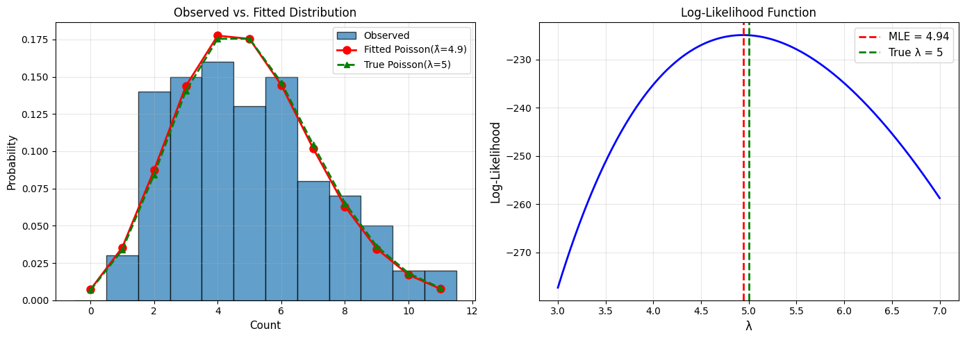
Example 3: Poisson Distribution#
Problem#
Count data (x_1, \ldots, x_n \sim \text{Poisson}(\lambda)). Estimate λ.
Solution#
PMF: (P(X=k) = \frac{\lambda^k e^{-\lambda}}{k!})
Log-likelihood: $\( \ell(\lambda) = \sum_{i=1}^{n}\left[x_i\log\lambda - \lambda - \log(x_i!)\right] \)$
Derivative: $\( \frac{d\ell}{d\lambda} = \frac{1}{\lambda}\sum_{i=1}^{n}x_i - n = 0 \)$
MLE: $\( \hat{\lambda}_{\text{MLE}} = \frac{1}{n}\sum_{i=1}^{n}x_i = \bar{x} \)$
The MLE is the sample mean!
Python Implementation#
import numpy as np
import matplotlib.pyplot as plt
from scipy import stats
from scipy.special import gammaln

np.random.seed(42)

# Generate Poisson data (e.g., number of customers per hour)
true_lambda = 5
n = 100
counts = np.random.poisson(true_lambda, n)

print("Poisson MLE Example")
print("="*70)
print(f"True λ: {true_lambda}")
print(f"Sample: {n} observations")
print(f"Sample mean: {np.mean(counts):.3f}")
print(f"Sample variance: {np.var(counts, ddof=1):.3f}")
print()

# MLE
lambda_mle = np.mean(counts)
print(f"MLE estimate: λ̂ = {lambda_mle:.3f}")
print()
# Log-likelihood function
def log_likelihood_poisson(lam, data):
    if lam <= 0:
        return -np.inf
    return np.sum(data * np.log(lam) - lam - gammaln(data + 1))
    return np.sum(data * np.log(lam) - lam - np.log(stats.factorial(data)))

# Plot
fig, (ax1, ax2) = plt.subplots(1, 2, figsize=(14, 5))

# Data distribution
max_count = counts.max()
ax1.hist(counts, bins=range(max_count+2), density=True, alpha=0.7,
         edgecolor='black', align='left', label='Observed')
x = np.arange(0, max_count+1)
ax1.plot(x, stats.poisson.pmf(x, lambda_mle), 'ro-', linewidth=2,
         markersize=8, label=f'Fitted Poisson(λ̂={lambda_mle:.1f})')
ax1.plot(x, stats.poisson.pmf(x, true_lambda), 'g^--', linewidth=2,
         markersize=6, label=f'True Poisson(λ={true_lambda})')
ax1.set_xlabel('Count', fontsize=11)
ax1.set_ylabel('Probability', fontsize=11)
ax1.set_title('Observed vs. Fitted Distribution', fontsize=12)
ax1.legend(fontsize=10)
ax1.grid(alpha=0.3)

# Likelihood function
lambda_values = np.linspace(3, 7, 1000)
log_likes = [log_likelihood_poisson(lam, counts) for lam in lambda_values]

ax2.plot(lambda_values, log_likes, 'b-', linewidth=2)
ax2.axvline(lambda_mle, color='red', linestyle='--', linewidth=2,
            label=f'MLE = {lambda_mle:.2f}')
ax2.axvline(true_lambda, color='green', linestyle='--', linewidth=2,
            label=f'True λ = {true_lambda}')
ax2.set_xlabel('λ', fontsize=12)
ax2.set_ylabel('Log-Likelihood', fontsize=12)
ax2.set_title('Log-Likelihood Function', fontsize=12)
ax2.legend(fontsize=11)
ax2.grid(alpha=0.3)

plt.tight_layout()
plt.savefig('poisson_mle.png', dpi=150, bbox_inches='tight')
plt.show()
Poisson MLE Example
======================================================================
True λ: 5
Sample: 100 observations
Sample mean: 4.940
Sample variance: 5.673

MLE estimate: λ̂ = 4.940
Properties of MLEs#
1. Consistency#
As (n \to \infty), (\hat{\theta}{\text{MLE}} \to \theta{\text{true}}) (in probability)
2. Asymptotic Normality#
For large n: $\( \hat{\theta}_{\text{MLE}} \sim N\left(\theta, \frac{1}{nI(\theta)}\right) \)$
where (I(\theta)) is the Fisher Information.
3. Efficiency#
MLEs achieve the Cramér-Rao lower bound - no unbiased estimator has smaller variance.
4. Invariance#
If (\hat{\theta}) is the MLE of θ, then (g(\hat{\theta})) is the MLE of (g(\theta)) for any function g.
Confidence Intervals from MLE#
Using Asymptotic Normality#
For large n: $\( \hat{\theta} \pm z_{\alpha/2} \cdot \text{SE}(\hat{\theta}) \)$
where SE is estimated from Fisher Information or observed information.
Profile Likelihood#
More accurate for small samples: $\( \{\theta: 2(\ell(\hat{\theta}) - \ell(\theta)) \leq \chi^2_{1,\alpha}\} \)$
Numerical MLE#
For complex models without closed-form solutions:
from scipy.optimize import minimize
import numpy as np

def neg_log_likelihood(params, data):
    # params = [mu, sigma], with sigma > 0
    mu, sigma = params
    if sigma <= 0 or not np.isfinite(sigma):
        return np.inf
    n = len(data)
    return n/2 * np.log(2*np.pi) + n/2 * np.log(sigma**2) + np.sum((data - mu)**2) / (2 * sigma**2)

# Use existing estimates from the notebook as starting values
initial_guess = [mu_mle, sigma_mle]

result = minimize(neg_log_likelihood, initial_guess, args=(data,), method='BFGS')

mle_params = result.x
print(f"MLE: {mle_params}")
print(f"Negative log-likelihood: {result.fun}")
print(f"Success: {result.success}")
MLE: [9.54905219 1.84856988]
Negative log-likelihood: 101.66754166036912
Success: True
Summary#
MLE Recipe#
Write likelihood: (L(\theta) = \prod f(x_i \mid \theta))
Take log: (\ell(\theta) = \sum \log f(x_i \mid \theta))
Differentiate: (\frac{d\ell}{d\theta} = 0)
Solve: Find (\hat{\theta}_{\text{MLE}})
Verify: Check second derivative or use numerical optimization
Common MLEs#
Distribution |
Parameter |
MLE |
|---|---|---|
Bernoulli(p) |
p |
k/n (sample proportion) |
Normal(μ, σ²) |
μ |
(\bar{x}) (sample mean) |
Normal(μ, σ²) |
σ² |
(\frac{1}{n}\sum(x_i-\bar{x})^2) |
Poisson(λ) |
λ |
(\bar{x}) (sample mean) |
Exponential(λ) |
λ |
(1/\bar{x}) |
Advantages of MLE#
✅ Optimal properties (consistency, efficiency)
✅ General method (works for any model)
✅ No prior distribution needed
✅ Widely used and understood
Limitations#
❌ Can be unstable with small samples
❌ May not exist or be unique
❌ Doesn’t incorporate prior knowledge
❌ Requires optimization for complex models