![]()
1.5 You Should#
This section summarizes the key concepts, definitions, and skills you should have mastered from Chapter 1.
1.5.1 Remember These Definitions#
Definition 1.1: Mean $\(\text{mean}(\{x\}) = \frac{1}{N} \sum_{i=1}^{N} x_i\)$
The mean is the average value of a dataset.
Definition 1.2: Standard Deviation $\(\text{std}(\{x\}) = \sqrt{\frac{1}{N} \sum_{i=1}^{N} (x_i - \text{mean}(\{x\}))^2}\)$
The standard deviation measures the typical deviation from the mean.
Definition 1.3: Variance $\(\text{var}(\{x\}) = \frac{1}{N} \sum_{i=1}^{N} (x_i - \text{mean}(\{x\}))^2 = (\text{std}(\{x\}))^2\)$
The variance is the square of the standard deviation.
Definition 1.4: Median
The median is the middle value when data is sorted. For even-length datasets, it’s the average of the two middle values.
Definition 1.5: Percentile
The k-th percentile is the value such that k% of the data is less than or equal to that value.
Definition 1.6: Quartiles
Q1 (first quartile): 25th percentile
Q2 (second quartile): 50th percentile (median)
Q3 (third quartile): 75th percentile
Definition 1.7: Interquartile Range (IQR) $\(\text{IQR} = Q3 - Q1\)$
The IQR measures the spread of the middle 50% of the data.
Definition 1.8: Standard Coordinates (Z-scores) $\(\hat{x}_i = \frac{x_i - \text{mean}(\{x\})}{\text{std}(\{x\})}\)$
Standard coordinates normalize data to have mean 0 and standard deviation 1.
Definition 1.9: Standard Normal Data
Data is standard normal if its histogram (with many data points) approximates: $\(y(x) = \frac{1}{\sqrt{2\pi}} e^{-x^2/2}\)$
Definition 1.10: Normal Data
Data is normal if it becomes standard normal after computing standard coordinates.
1.5.2 Remember These Terms#
Dataset: A collection of observations or measurements
Categorical data: Data that falls into discrete categories
Ordinal data: Categorical data that can be ordered
Continuous data: Data that can take any value in a range
Bar chart: Visualization showing category frequencies
Histogram: Visualization showing distribution of continuous data
Conditional histogram: Histogram for a subset of data
Location parameter: A measure of where data is centered (mean, median)
Scale parameter: A measure of data spread (standard deviation, IQR)
Outlier: An unusually extreme data value
Skewness: Asymmetry in the distribution of data
Right-skewed: Long right tail, mean > median
Left-skewed: Long left tail, mean < median
Mode: The peak of a histogram
Unimodal: One peak
Bimodal: Two peaks
Multimodal: Multiple peaks
Box plot: Visualization showing five-number summary
1.5.3 Remember These Facts#
Properties of the Mean#
Scaling data scales the mean: \(\text{mean}(\{kx_i\}) = k \cdot \text{mean}(\{x_i\})\)
Translating data translates the mean: \(\text{mean}(\{x_i + c\}) = \text{mean}(\{x_i\}) + c\)
Sum of deviations from mean is zero: \(\sum_{i=1}^{N} (x_i - \text{mean}(\{x_i\})) = 0\)
The mean minimizes sum of squared distances: \(\text{argmin}_a \sum_i (x_i - a)^2 = \text{mean}(\{x\})\)
Properties of Standard Deviation#
Translation doesn’t change std: \(\text{std}(\{x_i + c\}) = \text{std}(\{x_i\})\)
Scaling scales std: \(\text{std}(\{kx_i\}) = |k| \cdot \text{std}(\{x_i\})\)
At most \(\frac{1}{k^2}\) of data can be k or more standard deviations from the mean
At least one data point must be at least one standard deviation from the mean
Properties of Variance#
\(\text{var}(\{x + c\}) = \text{var}(\{x\})\)
\(\text{var}(\{kx\}) = k^2 \cdot \text{var}(\{x\})\)
Properties of Median#
\(\text{median}(\{x + c\}) = \text{median}(\{x\}) + c\)
\(\text{median}(\{kx\}) = k \cdot \text{median}(\{x\})\)
Median is robust to outliers
Properties of Standard Coordinates#
\(\text{mean}(\{\tilde{x}\}) = 0\)
\(\text{std}(\{\tilde{x}\}) = 1\)
Properties of Normal Data#
For normal data:
About 68% lies within 1 standard deviation of the mean
About 95% lies within 2 standard deviations of the mean
About 99.7% lies within 3 standard deviations of the mean
This is the 68-95-99.7 rule or empirical rule.
1.5.4 Be Able to#
Computation Skills#
Calculate mean, median, standard deviation, variance, and IQR for a dataset
Compute percentiles and quartiles
Convert data to standard coordinates (z-scores)
Identify outliers using the IQR method (values < Q1 - 1.5×IQR or > Q3 + 1.5×IQR)
Visualization Skills#
Create bar charts for categorical data
Create histograms for continuous data
Create conditional histograms to compare subgroups
Create box plots to compare distributions
Interpret these visualizations to understand data structure
Analysis Skills#
Identify whether data is skewed (left, right, or symmetric)
Determine if data is unimodal, bimodal, or multimodal
Choose appropriate summary statistics (mean vs. median, std vs. IQR)
Recognize when data appears to be normally distributed
Compare multiple datasets using appropriate visualizations
Conceptual Understanding#
Explain why mean is sensitive to outliers but median is not
Explain why standard deviation measures spread
Explain what standard coordinates achieve
Explain the relationship between histogram shape and summary statistics
Explain when to use different types of plots
Python Skills You Should Have#
import numpy as np
import matplotlib.pyplot as plt
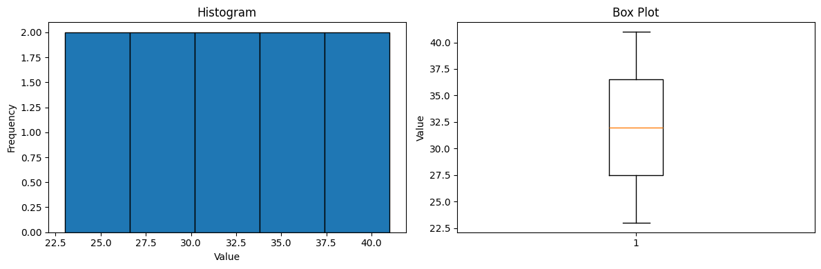
# Create sample data
data = np.array([23, 25, 27, 29, 31, 33, 35, 37, 39, 41])
# Compute summary statistics
print(f"Mean: {np.mean(data)}")
print(f"Median: {np.median(data)}")
print(f"Std Dev: {np.std(data)}")
print(f"Variance: {np.var(data)}")
print(f"Q1: {np.percentile(data, 25)}")
print(f"Q3: {np.percentile(data, 75)}")
print(f"IQR: {np.percentile(data, 75) - np.percentile(data, 25)}")
# Standardize
z_scores = (data - np.mean(data)) / np.std(data)
print(f"Z-scores: {z_scores}")
# Create visualizations
fig, axes = plt.subplots(1, 2, figsize=(12, 4))
# Histogram
axes[0].hist(data, bins=5, edgecolor='black')
axes[0].set_xlabel('Value')
axes[0].set_ylabel('Frequency')
axes[0].set_title('Histogram')
# Box plot
axes[1].boxplot(data)
axes[1].set_ylabel('Value')
axes[1].set_title('Box Plot')
plt.tight_layout()
plt.show()
Mean: 32.0
Median: 32.0
Std Dev: 5.744562646538029
Variance: 33.0
Q1: 27.5
Q3: 36.5
IQR: 9.0
Z-scores: [-1.5666989  -1.21854359 -0.87038828 -0.52223297 -0.17407766  0.17407766
  0.52223297  0.87038828  1.21854359  1.5666989 ]