7.1 Significance and P-Values

The Logic of Hypothesis Testing

The Setup

We have:

1. Data: Observations from an experiment or sample

2. Question: Is there a real effect, or just random variation?

The Framework

Null Hypothesis (H₀): The “nothing is happening” hypothesis

• Examples: “The drug has no effect”, “The coin is fair”, “Both designs convert equally”

Alternative Hypothesis (H₁ or Hₐ): What we’re trying to establish

• Examples: “The drug reduces blood pressure”, “The coin is biased”, “Design B converts better”

The Logic

1. Assume H₀ is true

2. Calculate: How likely is our observed data (or more extreme) under H₀?

3. Decide: If very unlikely, reject H₀ in favor of H₁

┌─────────────────────────────────────────────┐
│  If H₀ is true                              │
│  ↓                                          │
│  How probable is our observed result?       │
│  ↓                                          │
│  If very improbable → Reject H₀             │
│  If reasonably probable → Don't reject H₀   │
└─────────────────────────────────────────────┘

P-Values: The Core Concept

Definition

P-value: The probability of observing data as extreme as (or more extreme than) what we actually observed, assuming H₀ is true.

\[ \text{p-value} = P(\text{data as extreme or more} \mid H_0 \text{ is true}) \]

Interpretation

• Small p-value (typically < 0.05): Data is unlikely under H₀ → Evidence against H₀

• Large p-value: Data is consistent with H₀ → Insufficient evidence against H₀

Common Misconception

❌ WRONG: “p-value is the probability that H₀ is true” ✅ CORRECT: “p-value is the probability of our data (or more extreme) if H₀ were true”

Significance Levels

The α Threshold

Significance level (α): The threshold below which we reject H₀.

Common choices:

• α = 0.05 (5%) - standard in many fields

• α = 0.01 (1%) - more conservative

• α = 0.10 (10%) - more liberal

Decision Rule

• If p-value < α: Reject H₀ (result is “statistically significant”)

• If p-value ≥ α: Fail to reject H₀ (result is “not significant”)

Types of Errors

The Truth Table

	H₀ is True	H₀ is False
Reject H₀	Type I Error (α)	✓ Correct
Don’t Reject	✓ Correct	Type II Error (β)

Type I Error (False Positive)

• Definition: Rejecting H₀ when it’s actually true

• Probability: α (the significance level)

• Example: Concluding a drug works when it doesn’t

Type II Error (False Negative)

• Definition: Failing to reject H₀ when it’s actually false

• Probability: β (depends on effect size, sample size, α)

• Example: Missing a real drug effect

Power

Statistical Power = 1 - β = Probability of correctly rejecting false H₀

• High power (0.80 or more) is desirable

• Power increases with: larger effects, larger samples, higher α

Example 1: Coin Fairness Test

Problem

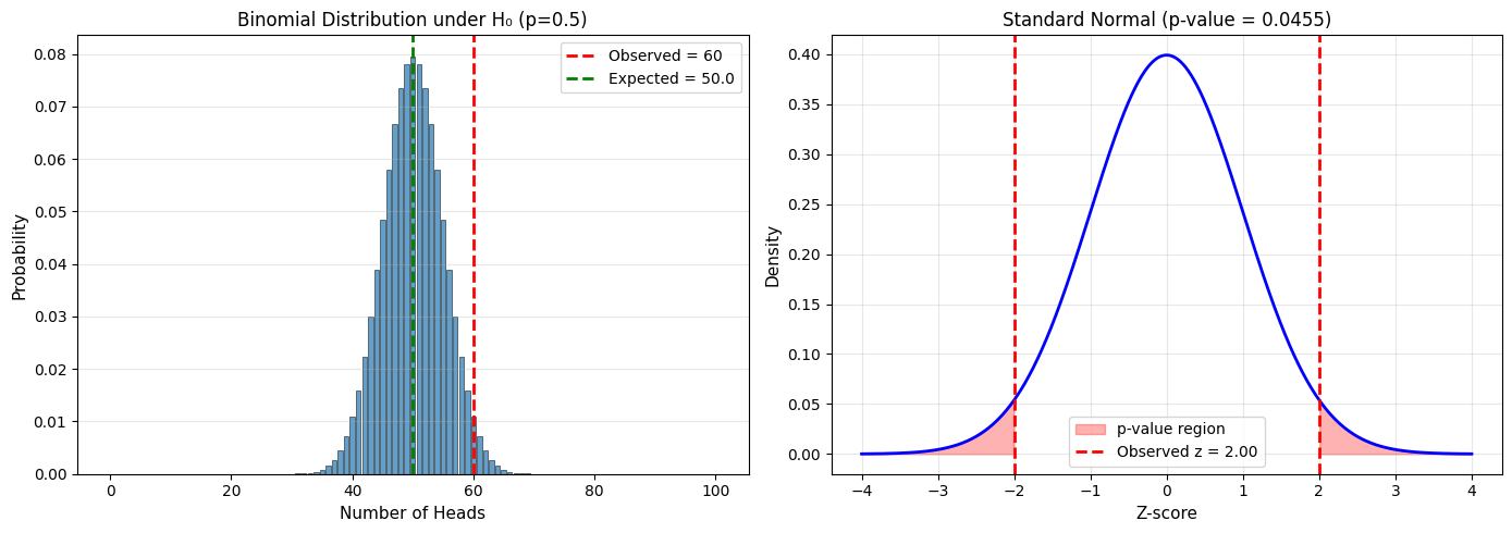
You flip a coin 100 times and get 60 heads. Is the coin fair?

Solution

import numpy as np
from scipy import stats
import matplotlib.pyplot as plt

# Data
n = 100
observed_heads = 60

# Hypotheses
print("H₀: The coin is fair (p = 0.5)")
print("H₁: The coin is not fair (p ≠ 0.5)")
print()

# Under H₀, number of heads ~ Binomial(n=100, p=0.5)
# For large n, approximate with normal distribution
p_null = 0.5
mean_null = n * p_null
std_null = np.sqrt(n * p_null * (1 - p_null))

print(f"Under H₀: Number of heads ~ N({mean_null}, {std_null:.2f}²)")
print()

# Z-score of observed result
z_score = (observed_heads - mean_null) / std_null
print(f"Observed: {observed_heads} heads")
print(f"Z-score: {z_score:.3f}")
print()

# P-value (two-tailed test)
p_value = 2 * (1 - stats.norm.cdf(abs(z_score)))
print(f"P-value (two-tailed): {p_value:.4f}")
print()

# Decision
alpha = 0.05
if p_value < alpha:
    print(f"Decision: p-value ({p_value:.4f}) < α ({alpha})")
    print("Reject H₀. Evidence suggests the coin is biased.")
else:
    print(f"Decision: p-value ({p_value:.4f}) ≥ α ({alpha})")
    print("Fail to reject H₀. Insufficient evidence of bias.")

# Visualization
fig, (ax1, ax2) = plt.subplots(1, 2, figsize=(14, 5))

# Left: Binomial distribution under H₀
x = np.arange(0, 101)
binom_probs = stats.binom.pmf(x, n, p_null)

ax1.bar(x, binom_probs, alpha=0.7, edgecolor='black', linewidth=0.5)
ax1.axvline(observed_heads, color='red', linestyle='--', linewidth=2, 
            label=f'Observed = {observed_heads}')
ax1.axvline(mean_null, color='green', linestyle='--', linewidth=2, 
            label=f'Expected = {mean_null}')
ax1.set_xlabel('Number of Heads', fontsize=11)
ax1.set_ylabel('Probability', fontsize=11)
ax1.set_title('Binomial Distribution under H₀ (p=0.5)', fontsize=12)
ax1.legend()
ax1.grid(alpha=0.3, axis='y')

# Right: Standard normal showing p-value
z_range = np.linspace(-4, 4, 1000)
norm_pdf = stats.norm.pdf(z_range)

ax2.plot(z_range, norm_pdf, 'b-', linewidth=2)
ax2.fill_between(z_range[z_range <= -abs(z_score)], 0, 
                  stats.norm.pdf(z_range[z_range <= -abs(z_score)]),
                  alpha=0.3, color='red', label='p-value region')
ax2.fill_between(z_range[z_range >= abs(z_score)], 0,
                  stats.norm.pdf(z_range[z_range >= abs(z_score)]),
                  alpha=0.3, color='red')
ax2.axvline(z_score, color='red', linestyle='--', linewidth=2,
            label=f'Observed z = {z_score:.2f}')
ax2.axvline(-z_score, color='red', linestyle='--', linewidth=2)
ax2.set_xlabel('Z-score', fontsize=11)
ax2.set_ylabel('Density', fontsize=11)
ax2.set_title(f'Standard Normal (p-value = {p_value:.4f})', fontsize=12)
ax2.legend()
ax2.grid(alpha=0.3)

plt.tight_layout()
plt.savefig('coin_test.png', dpi=150, bbox_inches='tight')
plt.show()

H₀: The coin is fair (p = 0.5)
H₁: The coin is not fair (p ≠ 0.5)

Under H₀: Number of heads ~ N(50.0, 5.00²)

Observed: 60 heads
Z-score: 2.000

P-value (two-tailed): 0.0455

Decision: p-value (0.0455) < α (0.05)
Reject H₀. Evidence suggests the coin is biased.

One-Tailed vs Two-Tailed Tests

Two-Tailed Test

H₁: Parameter ≠ value (different in either direction)

Example: “The coin is biased” (could be biased toward heads OR tails)

P-value includes both tails of the distribution.

One-Tailed Test

H₁: Parameter > value OR Parameter < value (specific direction)

Example: “The coin is biased toward heads” (only testing one direction)

P-value includes only one tail.

Choosing

• Two-tailed: Default choice, more conservative

• One-tailed: Use only when you have a strong directional hypothesis before seeing data

⚠️ Warning: Don’t switch to one-tailed after seeing your data - this is p-hacking!

Example 2: One-Sample Mean Test

Problem

A manufacturer claims light bulbs last 1000 hours on average. You test 25 bulbs: mean = 950 hours, std = 100 hours. Test the claim at α = 0.05.

Solution

import numpy as np
from scipy import stats

# Data
n = 25
sample_mean = 950
sample_std = 100
claim_mean = 1000
alpha = 0.05

print("Hypothesis Test: One-Sample t-test")
print("="*50)
print(f"H₀: μ = {claim_mean} (manufacturer's claim is true)")
print(f"H₁: μ ≠ {claim_mean} (manufacturer's claim is false)")
print(f"Significance level: α = {alpha}")
print()

# Test statistic
se = sample_std / np.sqrt(n)
t_stat = (sample_mean - claim_mean) / se
df = n - 1

print(f"Sample mean: {sample_mean}")
print(f"Sample std: {sample_std}")
print(f"Standard error: {se:.2f}")
print(f"t-statistic: {t_stat:.3f}")
print(f"Degrees of freedom: {df}")
print()

# P-value (two-tailed)
p_value = 2 * stats.t.cdf(t_stat, df)  # t_stat is negative
print(f"P-value: {p_value:.4f}")
print()

# Decision
if p_value < alpha:
    print(f"Decision: p-value ({p_value:.4f}) < α ({alpha})")
    print("Reject H₀. The manufacturer's claim is questionable.")
else:
    print(f"Decision: p-value ({p_value:.4f}) ≥ α ({alpha})")
    print("Fail to reject H₀. Insufficient evidence against the claim.")

# Using scipy's built-in function
t_stat_scipy, p_value_scipy = stats.ttest_1samp(
    np.random.normal(sample_mean, sample_std, n), claim_mean
)
print(f"\nVerification using scipy.stats.ttest_1samp:")
print(f"t-statistic: {t_stat:.3f}, p-value: {p_value:.4f}")

# Confidence interval
t_crit = stats.t.ppf(1 - alpha/2, df)
ci_lower = sample_mean - t_crit * se
ci_upper = sample_mean + t_crit * se

print(f"\n95% Confidence Interval: [{ci_lower:.1f}, {ci_upper:.1f}]")
print(f"Claimed value {claim_mean} is {'NOT' if claim_mean < ci_lower or claim_mean > ci_upper else ''} in the CI")

Hypothesis Test: One-Sample t-test
==================================================
H₀: μ = 1000 (manufacturer's claim is true)
H₁: μ ≠ 1000 (manufacturer's claim is false)
Significance level: α = 0.05

Sample mean: 950
Sample std: 100
Standard error: 20.00
t-statistic: -2.500
Degrees of freedom: 24

P-value: 0.0197

Decision: p-value (0.0197) < α (0.05)
Reject H₀. The manufacturer's claim is questionable.

Verification using scipy.stats.ttest_1samp:
t-statistic: -2.500, p-value: 0.0197

95% Confidence Interval: [908.7, 991.3]
Claimed value 1000 is NOT in the CI

The Relationship Between CIs and Hypothesis Tests

Key Insight

For a two-tailed test at significance level α:

Reject H₀: μ = μ₀ ⟺ μ₀ is outside the (1-α)×100% confidence interval

This provides an alternative way to test hypotheses using confidence intervals!

Power Analysis

What is Power?

Power = Probability of detecting an effect when it exists

Factors Affecting Power

1. Effect size: Larger effects → higher power

2. Sample size: Larger n → higher power

3. Significance level: Larger α → higher power (but more Type I errors)

4. Variance: Smaller σ → higher power

Example: Power Calculation

import numpy as np
from scipy import stats
import matplotlib.pyplot as plt

def calculate_power(n, effect_size, alpha=0.05, sigma=1):
    """
    Calculate power for one-sample t-test.
    
    effect_size: difference between true mean and null mean (in units of data)
    """
    # Non-centrality parameter
    ncp = effect_size / (sigma / np.sqrt(n))
    
    # Critical value
    df = n - 1
    t_crit = stats.t.ppf(1 - alpha/2, df)
    
    # Power (using non-central t-distribution)
    power = 1 - stats.nct.cdf(t_crit, df, ncp) + stats.nct.cdf(-t_crit, df, ncp)
    
    return power

# Example: Detect mean difference of 0.5σ
effect_sizes = [0.2, 0.5, 0.8]  # Small, medium, large (Cohen's d)
sample_sizes = np.arange(10, 201, 10)

fig, ax = plt.subplots(figsize=(10, 6))

for es in effect_sizes:
    powers = [calculate_power(n, es) for n in sample_sizes]
    ax.plot(sample_sizes, powers, linewidth=2, marker='o', 
            label=f'Effect size = {es} ({"small" if es==0.2 else "medium" if es==0.5 else "large"})')

ax.axhline(0.8, color='red', linestyle='--', linewidth=2, 
           label='Desired power = 0.80')
ax.set_xlabel('Sample Size (n)', fontsize=12)
ax.set_ylabel('Power', fontsize=12)
ax.set_title('Statistical Power vs. Sample Size\n(α = 0.05, two-tailed test)', fontsize=13)
ax.legend(fontsize=10)
ax.grid(alpha=0.3)
ax.set_ylim(0, 1)

plt.tight_layout()
plt.savefig('power_analysis.png', dpi=150, bbox_inches='tight')
plt.show()

print("Sample Size Needed for 80% Power:")
print("="*50)
for es in effect_sizes:
    for n in sample_sizes:
        if calculate_power(n, es) >= 0.8:
            print(f"Effect size {es}: n ≥ {n}")
            break

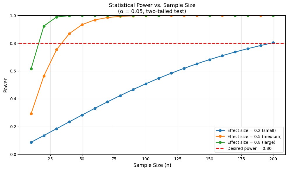
Sample Size Needed for 80% Power:
==================================================
Effect size 0.2: n ≥ 200
Effect size 0.5: n ≥ 40
Effect size 0.8: n ≥ 20

Summary

The Hypothesis Testing Recipe

1. State hypotheses: H₀ and H₁

2. Choose α: Significance level (usually 0.05)

3. Collect data: Sample and compute test statistic

4. Calculate p-value: Probability under H₀

5. Make decision: Reject H₀ if p-value < α

6. Interpret: In context of the problem

Key Formulas

One-sample t-test: $\( t = \frac{\bar{x} - \mu_0}{s/\sqrt{n}} \sim t_{n-1} \)$

Z-test (σ known): $\( z = \frac{\bar{x} - \mu_0}{\sigma/\sqrt{n}} \sim N(0,1) \)$

Important Points

✅ p-value measures evidence against H₀
✅ Small p-value → reject H₀
✅ “Not significant” ≠ “no effect”
✅ Statistical significance ≠ practical importance
✅ Always report effect sizes, not just p-values

❌ p-value ≠ P(H₀ is true)
❌ Don’t change hypotheses after seeing data
❌ Don’t confuse significance with importance
❌ Don’t p-hack (we’ll discuss this later!)