Statistics and probability relationship

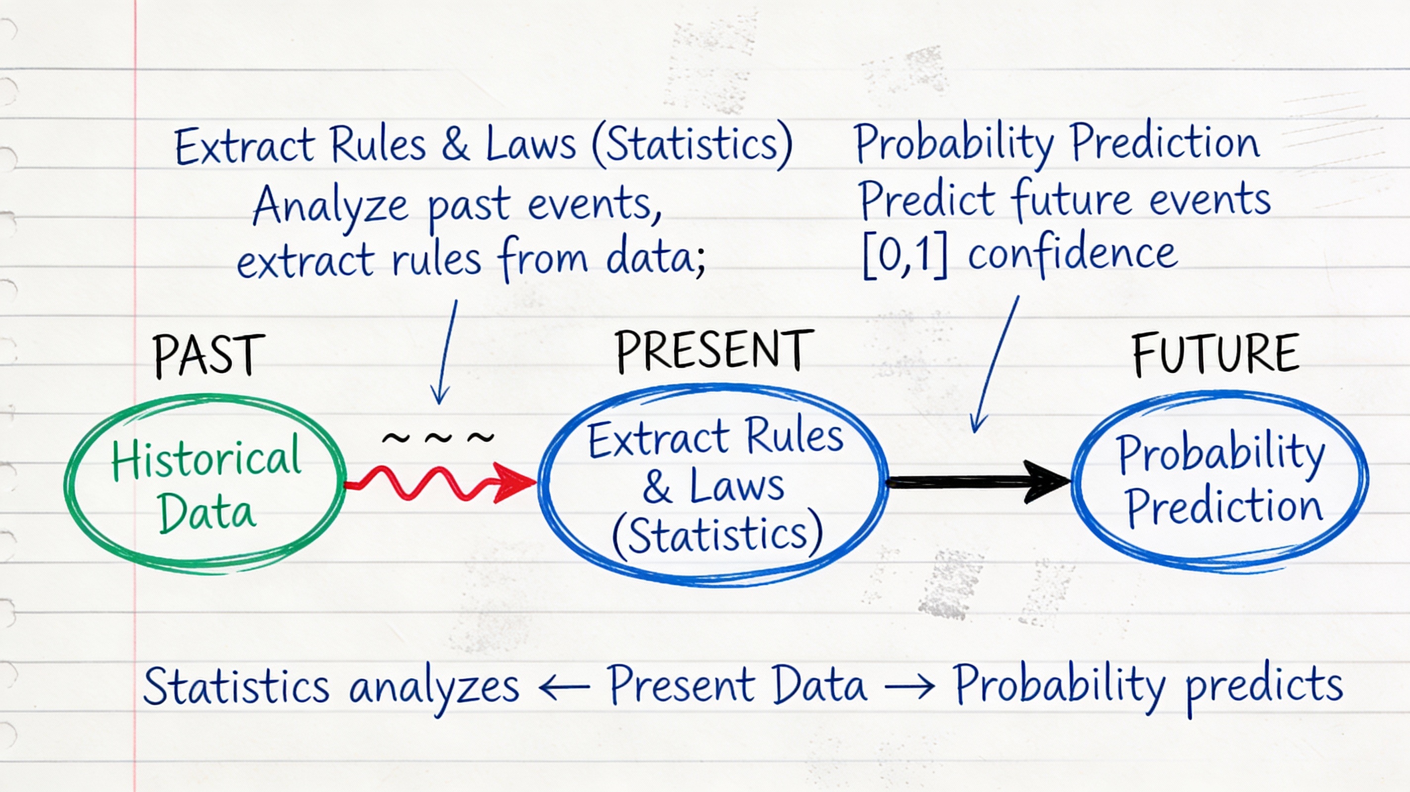
Before we can analyze data, we need to understand what data is and how we represent it.

What is a Dataset?

A dataset is a collection of descriptions of different instances of the same phenomenon. These descriptions could take a variety of forms, but it is important that they are descriptions of the same thing.

Examples of Datasets

1. Rainfall measurements: Daily rainfall in a garden over many years

2. Height measurements: Height of each person in a room

3. Family sizes: Number of children in each family on a block

4. Preferences: Whether 10 classmates prefer to be rich or famous

5. Student records: Test scores, attendance, demographics for students in a class

Key Characteristic

All items in a dataset must be:

• Descriptions of the same type of entity

• Measured or recorded in a consistent way

• Comparable to each other

❌ Not a dataset: [height of person 1, weight of person 2, age of person 3]
✅ Valid dataset: [height of person 1, height of person 2, height of person 3]

Lets see the operations on datasets

Union of Datasets

Given two datasets A and B, the union of A and B, denoted as A ∪ B, is a dataset that contains all the unique elements from both A and B.

A={1,2,3}
B={3,4,5}
print("A ∪ B =", A.union(B))

A ∪ B = {1, 2, 3, 4, 5}

Intersection of Datasets

Given two datasets A and B, the intersection of A and B, denoted as A ∩ B, is a dataset that contains only the elements that are present in both A and B.

print("A ∩ B =", A.intersection(B))

A ∩ B = {3}

Difference of Datasets

Given two datasets A and B, the difference of A and B, denoted as A - B, is a dataset that contains the elements that are in A but not in B.

print("A - B =", A.difference(B))

A - B = {1, 2}

Universal Set \(\Omega\)

In set theory, the universal set, often denoted by the symbol \(\Omega\) (omega), is the set that contains all the objects or elements under consideration for a particular discussion or problem. It serves as a reference point for defining other sets and their relationships. For example, if we are discussing the properties of natural numbers, the universal set \(\Omega\) would include all natural numbers: {0, 1, 2, 3, …}. If we are discussing the properties of geometric shapes, the universal set \(\Omega\) might include all possible geometric shapes. The universal set is important because it provides a context for understanding subsets, complements, and other set operations. Any set discussed within a particular context is considered a subset of the universal set \(\Omega\).

Complement of a Dataset

Given a dataset A and the universal set Ω, the complement of A, denoted as A’, is the dataset that contains all the elements that are in Ω but not in A.

omg = {1,2,3,4,5}
C = {2,3}
C_complement = omg.difference(C)
print("The complement of C is:", C_complement)

The complement of C is: {1, 4, 5}

Disjoint Datasets

Two datasets A and B are said to be disjoint if they have no elements in common. In other words, their intersection is the empty set. For example, if:

• Dataset A = {1, 2, 3}

• Dataset B = {4, 5, 6}

Then, A and B are disjoint because: A ∩ B = {} (the empty set)

Data Items and D-Tuples

A dataset consists of \(N\) data items, where each data item is a d-tuple - an ordered list of \(d\) elements.

Notation Conventions

• \(N\): Number of items in the dataset (always)

• \(d\): Number of elements in each tuple (always the same for all tuples)

• \(\{x\}\): The entire dataset

• \(x_i\): The \(i\)-th data item

• \(x_i^{(j)}\): The \(j\)-th component of the \(i\)-th data item

Example: Students Dataset

Consider 5 students with (height in cm, weight in kg, age in years):

Student	Height	Weight	Age
\(x_1\)	165	55	20
\(x_2\)	170	62	21
\(x_3\)	168	58	20
\(x_4\)	175	70	22
\(x_5\)	172	65	21

Here:

• \(N = 5\) (five students)

• \(d = 3\) (three measurements per student)

• \(x_1 = (165, 55, 20)\) (first student’s data)

• \(x_3^{(2)} = 58\) (third student’s weight)

# Example dataset: measurements of students
# Each student has three measurements: height (cm), weight (kg), age (years)
data = [
    (165, 55, 20),  # Student 1
    (170, 70, 22),  # Student 2
    (180, 80, 21),  # Student 3
    (175, 65, 23),  # Student 4
]
# Number of students (n) and measurements per student (d)
n = len(data)
d = len(data[0]) if n > 0 else 0    
print(f"Number of students: {n}, Number of measurements per student: {d}")  
# Accessing specific data points
x1 = data[0]  # First student's data
x3_weight = data[2][1]  # Third student's weight
print(f"First student's data: {x1}")
print(f"Third student's weight: {x3_weight} kg")   

Number of students: 4, Number of measurements per student: 3
First student's data: (165, 55, 20)
Third student's weight: 80 kg

Types of Data

Data comes in different types, each requiring different analysis techniques.

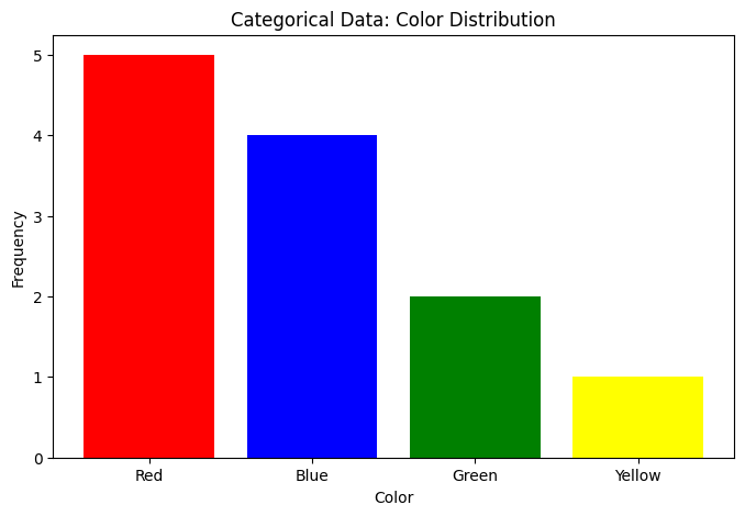
1. Categorical Data

Categorical data consists of values from a fixed set of categories with no inherent numerical meaning.

Examples:

• Gender: {Male, Female, Other}

• Color: {Red, Blue, Green, Yellow}

• Country: {USA, Canada, Mexico, …}

• Yes/No responses

Characteristics:

• Cannot meaningfully compute mean or standard deviation

• Can count frequencies

• Can compute mode (most common category)

• Use bar charts for visualization

import numpy as np
import matplotlib.pyplot as plt
from collections import Counter

# Categorical data example
colors = ['Red', 'Blue', 'Red', 'Green', 'Blue', 'Red', 
          'Yellow', 'Blue', 'Red', 'Blue', 'Green', 'Red']

# Count frequencies
counts = Counter(colors)
print("Frequencies:", counts)
print("Mode:", counts.most_common(1)[0][0])

# Visualize
categories = list(counts.keys())
frequencies = list(counts.values())

plt.figure(figsize=(8, 5))
plt.bar(categories, frequencies, color=['red', 'blue', 'green', 'yellow'])
plt.xlabel('Color')
plt.ylabel('Frequency')
plt.title('Categorical Data: Color Distribution')
plt.show()

Frequencies: Counter({'Red': 5, 'Blue': 4, 'Green': 2, 'Yellow': 1})
Mode: Red

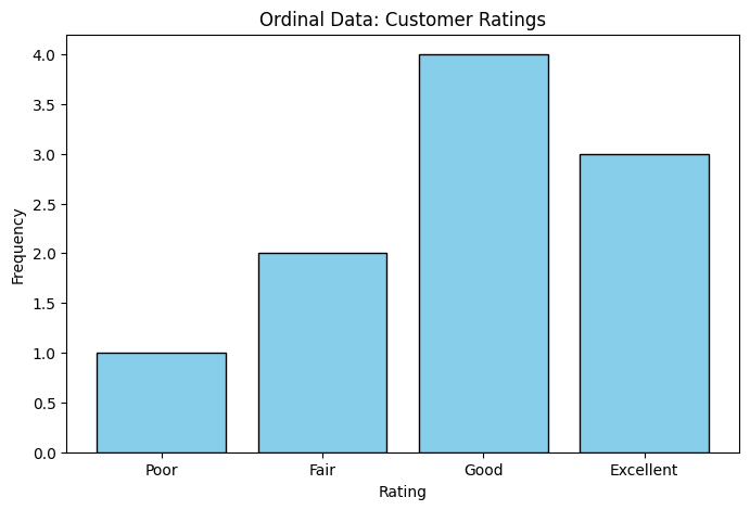
2. Ordinal Data

Ordinal data consists of categories with a meaningful order or ranking, but the intervals between categories are not necessarily equal.

Examples:

• Education Level: {High School, Bachelor’s, Master’s, PhD}

• Satisfaction Rating: {Very Unsatisfied, Unsatisfied, Neutral, Satisfied, Very Satisfied}

• Military Ranks: {Private, Corporal, Sergeant, Lieutenant, Captain}

Characteristics:

• Can determine order (e.g., Master’s > Bachelor’s)

• Cannot compute mean or standard deviation meaningfully

• Can compute median and mode

• Use bar charts or ordered plots for visualization

# Ordinal data example
ratings = ['Good', 'Excellent', 'Fair', 'Good', 'Poor', 
           'Excellent', 'Good', 'Good', 'Fair', 'Excellent']

# Define order
order = ['Poor', 'Fair', 'Good', 'Excellent']

# Map to numbers for analysis
rating_map = {rating: i for i, rating in enumerate(order)}
numeric_ratings = [rating_map[r] for r in ratings]

print(f"Median rating: {order[int(np.median(numeric_ratings))]}")
print(f"Mode rating: {Counter(ratings).most_common(1)[0][0]}")

# Visualize
rating_counts = Counter(ratings)
ordered_counts = [rating_counts[r] for r in order]

plt.figure(figsize=(8, 5))
plt.bar(order, ordered_counts, color='skyblue', edgecolor='black')
plt.xlabel('Rating')
plt.ylabel('Frequency')
plt.title('Ordinal Data: Customer Ratings')
plt.show()

Median rating: Good
Mode rating: Good

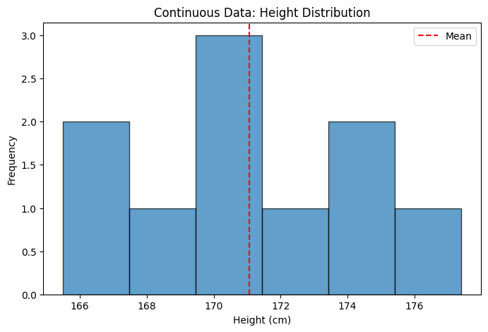
3. Continuous Data

Continuous data consists of numerical values that can take any value within a range. These values have meaningful intervals and ratios.

Examples:

• Height in centimeters

• Weight in kilograms

• Temperature in degrees Celsius

• Time in seconds

Characteristics:

• Can compute mean, median, mode, standard deviation

• Can perform arithmetic operations

• Use histograms, box plots, scatter plots for visualization

# Continuous data example
heights = np.array([165.5, 170.2, 168.7, 175.1, 172.3, 
                    169.8, 173.6, 177.4, 171.2, 166.9])

print(f"Mean height: {np.mean(heights):.2f} cm")
print(f"Median height: {np.median(heights):.2f} cm")
print(f"Std deviation: {np.std(heights):.2f} cm")

plt.figure(figsize=(8, 5))
plt.hist(heights, bins=6, edgecolor='black', alpha=0.7)
plt.xlabel('Height (cm)')
plt.ylabel('Frequency')
plt.title('Continuous Data: Height Distribution')
plt.axvline(np.mean(heights), color='r', linestyle='--', label='Mean')
plt.legend()
plt.show()

Mean height: 171.07 cm
Median height: 170.70 cm
Std deviation: 3.47 cm

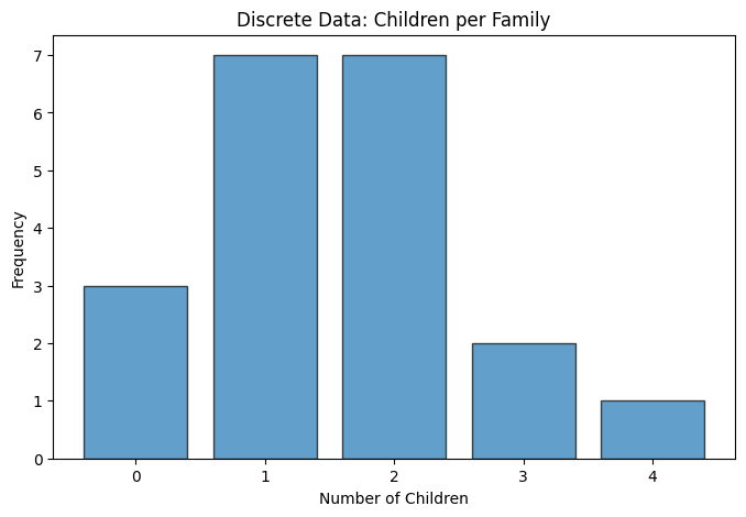
4. Discrete Data

Discrete data consists of numerical values that can only take specific, separate values (often integers). There are gaps between possible values.

Examples:

• Number of children in a family

• Number of cars in a parking lot

• Number of students in a class

• Number of goals scored in a soccer match

Characteristics:

• Can compute mean, median, mode, standard deviation

• Can perform arithmetic operations

• Use bar charts or dot plots for visualization

# Discrete data example
children_per_family = np.array([0, 1, 2, 1, 3, 2, 1, 0, 2, 1, 
                                 2, 4, 1, 2, 3, 1, 2, 0, 1, 2])

print(f"Mean: {np.mean(children_per_family):.2f} children")
print(f"Median: {np.median(children_per_family):.0f} children")
print(f"Mode: {Counter(children_per_family).most_common(1)[0][0]} children")

plt.figure(figsize=(8, 5))
values, counts = np.unique(children_per_family, return_counts=True)
plt.bar(values, counts, edgecolor='black', alpha=0.7)
plt.xlabel('Number of Children')
plt.ylabel('Frequency')
plt.title('Discrete Data: Children per Family')
plt.xticks(values)
plt.show()

Mean: 1.55 children
Median: 2 children
Mode: 1 children

Dealing with missing data

When dealing with missing data in datasets, there are several strategies you can employ to handle the gaps effectively. Here are some common approaches:

1. Remove Missing Data: If the amount of missing data is small, you can simply remove the records with missing values. However, this may lead to loss of valuable information if a significant portion of the dataset is affected.

2. Imputation: Replace missing values with estimated values based on other available data. Common imputation methods include:

   • Mean/Median/Mode Imputation: Replace missing values with the mean, median, or mode of the respective feature.

   • Regression Imputation: Use regression models to predict and fill in missing values based on other features.

   • K-Nearest Neighbors (KNN) Imputation: Use the values from similar instances (neighbors) to fill in missing data.

3. Use Algorithms that Handle Missing Data: Some machine learning algorithms can handle missing data internally, such as decision trees and random forests.

import pandas as pd

# Dataset with missing values
data = pd.DataFrame({
    'Height': [165, 170, 168, np.nan, 172],
    'Weight': [55, 62, np.nan, 70, 65],
    'Score': [85, 90, 88, 92, np.nan]
})

print("Original data:")
print(data)
print(f"\nMissing values:\n{data.isna().sum()}")

# Strategy 1: Drop rows with any missing
data_dropped = data.dropna()
print(f"\nAfter dropping: {len(data_dropped)} rows")

# Strategy 2: Fill with mean
data_filled = data.fillna(data.mean())
print("\nAfter filling with mean:")
print(data_filled)

Original data:
   Height  Weight  Score
0   165.0    55.0   85.0
1   170.0    62.0   90.0
2   168.0     NaN   88.0
3     NaN    70.0   92.0
4   172.0    65.0    NaN

Missing values:
Height    1
Weight    1
Score     1
dtype: int64

After dropping: 2 rows

After filling with mean:
   Height  Weight  Score
0  165.00    55.0  85.00
1  170.00    62.0  90.00
2  168.00    63.0  88.00
3  168.75    70.0  92.00
4  172.00    65.0  88.75

Loading and Exploring Datasets

Reading CSV Files

import pandas as pd
import io

# Read CSV
df = pd.read_csv('https://raw.githubusercontent.com/chebil/stat/main/part1/data.csv')

# Basic exploration
print(df.head())  # First 5 rows
print(df.info())  # Data types and missing values
print(df.describe())  # Summary statistics

      Name  Age  Score
0    Alice   20     85
1      Bob   21     90
2  Charlie   20     88
3    David   22     92
4      Eve   21     87
<class 'pandas.core.frame.DataFrame'>
RangeIndex: 5 entries, 0 to 4
Data columns (total 3 columns):
 #   Column  Non-Null Count  Dtype 
---  ------  --------------  ----- 
 0   Name    5 non-null      object
 1   Age     5 non-null      int64 
 2   Score   5 non-null      int64 
dtypes: int64(2), object(1)
memory usage: 252.0+ bytes
None
            Age      Score
count   5.00000   5.000000
mean   20.80000  88.400000
std     0.83666   2.701851
min    20.00000  85.000000
25%    20.00000  87.000000
50%    21.00000  88.000000
75%    21.00000  90.000000
max    22.00000  92.000000

Reading from dictionary

import pandas as pd
import numpy as np

# From dictionary
data = {
    'Name': ['Alice', 'Bob', 'Charlie', 'David'],
    'Age': [20, 21, 20, 22],
    'Score': [85, 90, 88, 92]
}
df = pd.DataFrame(data)

print(df)
print(f"\nDataset has {len(df)} items (N = {len(df)})")
print(f"Each item has {len(df.columns)} features (d = {len(df.columns)})")

      Name  Age  Score
0    Alice   20     85
1      Bob   21     90
2  Charlie   20     88
3    David   22     92

Dataset has 4 items (N = 4)
Each item has 3 features (d = 3)

Common Data Sources

1. Surveys and Questionnaires

• Collect specific information from individuals

• Often mix categorical and continuous data

• Example: Customer satisfaction surveys

2. Sensors and Measurements

• Automated data collection

• Usually continuous or discrete

• Example: Temperature sensors, GPS coordinates

3. Databases and Records

• Existing organizational data

• Structured format

• Example: Hospital records, sales transactions

4. Web Scraping

• Extract data from websites

• Requires cleaning and processing

• Example: Product prices, social media data

5. Public Datasets

• Freely available for research and education

• Often well-documented

• Examples:

  • UCI Machine Learning Repository

  • Kaggle Datasets

  • Data.gov

Best Practices for Working with Datasets

1. Always Explore First

# Check first few rows
print(df.head())

# Check data types
print(df.dtypes)

# Check for missing values
print(df.isna().sum())

# Summary statistics
print(df.describe())

      Name  Age  Score
0    Alice   20     85
1      Bob   21     90
2  Charlie   20     88
3    David   22     92
Name     object
Age       int64
Score     int64
dtype: object
Name     0
Age      0
Score    0
dtype: int64
             Age      Score
count   4.000000   4.000000
mean   20.750000  88.750000
std     0.957427   2.986079
min    20.000000  85.000000
25%    20.000000  87.250000
50%    20.500000  89.000000
75%    21.250000  90.500000
max    22.000000  92.000000

2. Visualize Early

• Plot histograms for continuous variables

• Create bar charts for categorical variables

• Look for outliers and patterns

3. Document Your Data

• What does each column represent?

• What are the units?

• When/how was data collected?

• Are there known issues?

4. Clean Your Data

• Handle missing values

• Remove duplicates

• Fix data type issues

• Deal with outliers

# Example cleaning pipeline
df_clean = df.copy()

# Remove duplicates
df_clean = df_clean.drop_duplicates()

# Handle missing values (only for numeric columns)
numeric_cols = df_clean.select_dtypes(include=[np.number]).columns
df_clean[numeric_cols] = df_clean[numeric_cols].fillna(df_clean[numeric_cols].mean())

# Convert types if needed
df_clean['Age'] = df_clean['Age'].astype(int)

print(f"Cleaned: {len(df)} → {len(df_clean)} rows")

Cleaned: 4 → 4 rows

Summary

Key takeaways:

1. Dataset: Collection of descriptions of the same phenomenon

2. N data items, each with d elements

3. Four data types: Categorical, Ordinal, Discrete, Continuous

4. Different types require different analyses

5. Missing data is common - have a strategy to handle it

6. Always explore and visualize before analyzing