![]()
3.2 Events#
Assume we run an experiment and get an outcome. We know what the outcome is—that’s the whole point of a sample space. This means we can tell whether the outcome we get belongs to some particular known set of outcomes. We just look in the set and see if our outcome is there.
For example, we might roll a die and ask “what is the probability of getting an even number?” We would like our probability models to be able to predict the probability of sets of outcomes.
Definition 3.2: Event#
An event is a set of outcomes. We will usually write events as sets (e.g., \(E\)).
Assume we are given a discrete sample space \(\Omega\). A natural choice of an event space is the collection of all subsets of \(\Omega\).
Key Properties#
The set of all outcomes, \(\Omega\), must be an event with \(P(\Omega) = 1\)
The empty set \(\emptyset\) is an event with \(P(\emptyset) = 0\)
Any given outcome must be an event
If \(E\) and \(F\) are disjoint events, then \(P(E \cup F) = P(E) + P(F)\)
Useful Facts 3.1: Basic Properties#
Property 1: Bounded Probabilities#
Property 2: Certainty#
Property 3: Additivity for Disjoint Events#
For disjoint events \(A_i\) (where \(A_i \cap A_j = \emptyset\) when \(i \neq j\)):
3.2.1 Computing Event Probabilities by Counting#
For equally likely outcomes:
Remember This
Compute probabilities of events by counting outcomes when all outcomes are equally likely.
Worked Example 3.5: Odd Numbers with Fair Dice#
Problem: Throw a fair six-sided die twice, then add the numbers. What is the probability of getting an odd number?
Solution: There are 36 outcomes, each with probability \(\frac{1}{36}\). Eighteen give an odd number, so:
import itertools
import numpy as np
import matplotlib.pyplot as plt

# Generate all outcomes
dice_outcomes = list(itertools.product(range(1, 7), repeat=2))
sums = [d1 + d2 for d1, d2 in dice_outcomes]
odd_sums = [s for s in sums if s % 2 == 1]

print(f"Total outcomes: {len(dice_outcomes)}")
print(f"Odd sums: {len(odd_sums)} ({len(odd_sums)/36:.1%})")
print(f"Even sums: {36-len(odd_sums)} ({(36-len(odd_sums))/36:.1%})")
Total outcomes: 36
Odd sums: 18 (50.0%)
Even sums: 18 (50.0%)
Worked Example 3.6: Numbers Divisible by Five#
Problem: Throw two fair dice, add the numbers. What is \(P(\text{divisible by 5})\)?
Solution: Spots must add to 5 or 10.
4 ways to get 5: \((1,4), (2,3), (3,2), (4,1)\)
3 ways to get 10: \((4,6), (5,5), (6,4)\)
div_by_5 = [(i,j) for i,j in dice_outcomes if (i+j) % 5 == 0]
print(f"Outcomes: {div_by_5}")
print(f"P(divisible by 5) = {len(div_by_5)}/36 = {len(div_by_5)/36:.4f}")
Outcomes: [(1, 4), (2, 3), (3, 2), (4, 1), (4, 6), (5, 5), (6, 4)]
P(divisible by 5) = 7/36 = 0.1944
Worked Example 3.7: Children1#
Problem: Couple has 3 children. Boys and girls equally likely. Let \(B_i\) = event of \(i\) boys, \(C\) = more girls than boys. Find \(P(B_1)\) and \(P(C)\).
Solution: 8 outcomes, all equally likely:
\(\{BBB, BBG, BGB, BGG, GBB, GBG, GGB, GGG\}\)
3 outcomes have 1 boy: \(P(B_1) = \frac{3}{8}\)
4 outcomes have more girls: \(P(C) = \frac{1}{2}\)
Worked Example 3.8: Fictitious Outcomes#
Problem: Have children until first girl or until 3. Find \(P(B_1)\) and \(P(C)\).
Solution: Use fictitious later births (lowercase):
1 girl: \(\{Gbb, Gbg, Ggb, Ggg\}\) → \(P = \frac{1}{2}\)
Boy then girl: \(\{BGb, BGg\}\) → \(P = \frac{1}{4}\)
2 boys then girl: \(\{BBG\}\) → \(P = \frac{1}{8}\)
3 boys: \(\{BBB\}\) → \(P = \frac{1}{8}\)
Thus: \(P(B_1) = \frac{1}{4}\), \(P(C) = \frac{1}{2}\)
Permutations and Combinations#
Permutations#
Number of ways to order \(N\) items: \(N!\)
Combinations#
Choose \(k\) from \(N\) (order doesn’t matter): $\(\binom{N}{k} = \frac{N!}{k!(N-k)!}\)$
Worked Example 3.9: Card Hands (Ordered)#
Problem: Draw 7 cards. Probability of 2-8 hearts in that order?
Solution:
Total orderings: \(52!\)
Favorable: first 7 are 2-8 hearts in order, remaining 45 arbitrary: \(45!\)
Worked Example 3.10: Card Hands (Unordered)#
Problem: Draw 7 cards. Probability of 2-8 hearts in any order?
Solution Method 1: $\(P = \frac{7! \cdot 45!}{52!}\)$
Method 2 (combinations):
Total hands: \(\binom{52}{7}\)
Favorable: 1
from scipy.special import comb
n_hands = comb(52, 7, exact=True)
print(f"Total 7-card hands: {n_hands:,}")
print(f"P(2-8 hearts any order) = 1/{n_hands:,} = {1/n_hands:.4e}")
Total 7-card hands: 133,784,560
P(2-8 hearts any order) = 1/133,784,560 = 7.4747e-09
Worked Example 3.11: Any Suit#
Problem: Draw 7 cards. Probability of 2-8 of any suit?
Solution: Each card can be any of 4 suits: $\(P = \frac{4^7}{\binom{52}{7}} = \frac{16384}{133784560} \approx 0.0001\)$
3.2.2 The Probability of Events#
The Size Analogy#
Think of probability as “size” relative to \(\Omega\) (which has size 1).
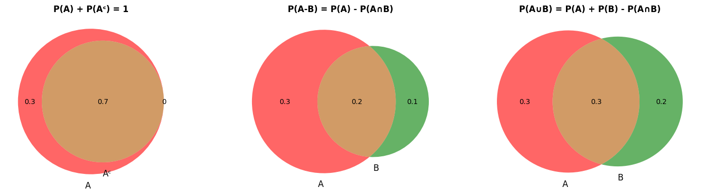
Venn Diagrams help visualize:
Complement: \(A\) and \(A^c\) partition \(\Omega\) $\(P(A) + P(A^c) = 1\)$
Set Difference: Part of \(A\) not in \(B\) $\(P(A - B) = P(A) - P(A \cap B)\)$
Union: Add sizes, subtract intersection $\(P(A \cup B) = P(A) + P(B) - P(A \cap B)\)$
from matplotlib_venn import venn2
import matplotlib.pyplot as plt

fig, axes = plt.subplots(1, 3, figsize=(15, 4))

# Complement
ax = axes[0]
venn2(subsets=(0.3, 0, 0.7), set_labels=('A', 'Aᶜ'), ax=ax, alpha=0.6)
ax.set_title('P(A) + P(Aᶜ) = 1', fontweight='bold')

# Set difference
ax = axes[1]
venn2(subsets=(0.3, 0.1, 0.2), set_labels=('A', 'B'), ax=ax, alpha=0.6)
ax.set_title('P(A-B) = P(A) - P(A∩B)', fontweight='bold')

# Union
ax = axes[2]
venn2(subsets=(0.3, 0.2, 0.3), set_labels=('A', 'B'), ax=ax, alpha=0.6)
ax.set_title('P(A∪B) = P(A) + P(B) - P(A∩B)', fontweight='bold')

plt.tight_layout()
plt.show()
Useful Facts 3.2: Properties of Events#
Property |
Formula |
|---|---|
Complement |
\(P(A^c) = 1 - P(A)\) |
Empty set |
\(P(\emptyset) = 0\) |
Set difference |
\(P(A - B) = P(A) - P(A \cap B)\) |
Union |
\(P(A \cup B) = P(A) + P(B) - P(A \cap B)\) |
Proofs#
Prop: \(P(A^c) = 1 - P(A)\)
Proof: \(A^c\) and \(A\) are disjoint, and \(A^c \cup A = \Omega\), so: $\(P(A^c) + P(A) = P(\Omega) = 1\)$
Prop: \(P(A \cup B) = P(A) + P(B) - P(A \cap B)\)
Proof: \(A \cup B = A \cup (B - A)\) where \(A\) and \(B-A\) are disjoint: $\(P(A \cup B) = P(A) + P(B - A)\)$
Now \(P(B - A) = P(B) - P(A \cap B)\), giving the result. \(\square\)
3.2.3 Computing with Set Operations#
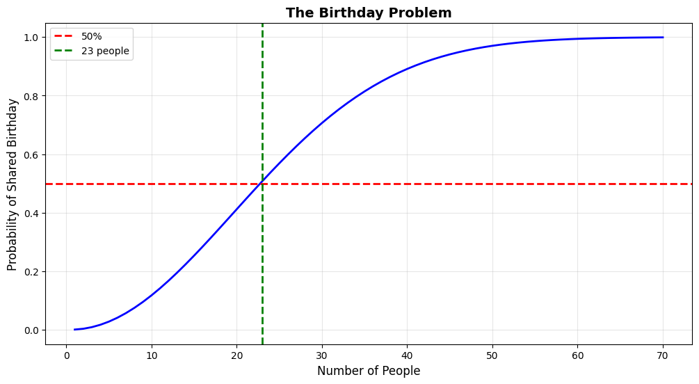
Worked Example 3.12: The Birthday Problem#
Problem: In a room of 30 people, what is \(P(\text{shared birthday})\)?
Solution: Use complement: $\(P(\text{shared}) = 1 - P(\text{all different})\)$
71% chance with just 30 people!
def birthday_prob(n, days=365):
    if n > days:
        return 1.0
    prob_all_diff = 1.0
    for i in range(n):
        prob_all_diff *= (days - i) / days
    return 1 - prob_all_diff

for n in [10, 20, 23, 30, 50]:
    print(f"{n:2d} people: P(shared) = {birthday_prob(n):.4f}")

# Find n for P > 50%
for n in range(1, 100):
    if birthday_prob(n) > 0.5:
        print(f"\nSmallest n for P>50%: {n}")
        break
10 people: P(shared) = 0.1169
20 people: P(shared) = 0.4114
23 people: P(shared) = 0.5073
30 people: P(shared) = 0.7063
50 people: P(shared) = 0.9704

Smallest n for P>50%: 23
Visualization:
n_values = range(1, 71)
probs = [birthday_prob(n) for n in n_values]

plt.figure(figsize=(12, 6))
plt.plot(n_values, probs, linewidth=2, color='blue')
plt.axhline(y=0.5, color='red', linestyle='--', linewidth=2, label='50%')
plt.axvline(x=23, color='green', linestyle='--', linewidth=2, label='23 people')
plt.xlabel('Number of People', fontsize=12)
plt.ylabel('Probability of Shared Birthday', fontsize=12)
plt.title('The Birthday Problem', fontsize=14, fontweight='bold')
plt.grid(True, alpha=0.3)
plt.legend()
plt.show()
Worked Example 3.13: Your Birthday#
Problem: In a room of 30 people, what is \(P(\text{someone shares YOUR birthday})\)?
Solution: $\(P(\text{winning}) = 1 - \left(\frac{364}{365}\right)^{29} \approx 0.077\)$
Only 7.7%! Very different from 71% in Example 3.12.
prob_your_bday = 1 - (364/365)**29
print(f"P(someone shares YOUR birthday) = {prob_your_bday:.4f}")
print(f"vs P(any two share) = {birthday_prob(30):.4f}")
print(f"Ratio: {birthday_prob(30)/prob_your_bday:.1f}x")
P(someone shares YOUR birthday) = 0.0765
vs P(any two share) = 0.7063
Ratio: 9.2x
Worked Example 3.14: Dice Divisibility#
Problem: Roll two dice, add spots. Find \(P(\text{div by 2 but not 5})\).
Solution: Let \(D_n\) = “divisible by \(n\)”
\(P(D_2) = \frac{1}{2}\) (symmetry)
\(D_2 \cap D_5\) = divisible by 10: outcomes \((4,6), (5,5), (6,4)\)
\(P(D_2 \cap D_5) = \frac{3}{36}\)
Worked Example 3.15: Union Example#
Problem: Roll two dice. Find \(P(\text{div by 2 OR 5})\).
Solution: $\(P(D_2 \cup D_5) = P(D_2) + P(D_5) - P(D_2 \cap D_5)\)\( \)\(= \frac{18}{36} + \frac{7}{36} - \frac{3}{36} = \frac{22}{36}\)$
dice = [(i,j) for i in range(1,7) for j in range(1,7)]
d2 = [(i,j) for i,j in dice if (i+j)%2==0]
d5 = [(i,j) for i,j in dice if (i+j)%5==0]
d2_and_d5 = [(i,j) for i,j in dice if (i+j)%10==0]
d2_or_d5 = [(i,j) for i,j in dice if (i+j)%2==0 or (i+j)%5==0]

print(f"P(D₂) = {len(d2)}/36 = {len(d2)/36:.4f}")
print(f"P(D₅) = {len(d5)}/36 = {len(d5)/36:.4f}")
print(f"P(D₂∩D₅) = {len(d2_and_d5)}/36 = {len(d2_and_d5)/36:.4f}")
print(f"P(D₂∪D₅) = {len(d2_or_d5)}/36 = {len(d2_or_d5)/36:.4f}")
print(f"Check: {len(d2)/36 + len(d5)/36 - len(d2_and_d5)/36:.4f}")
P(D₂) = 18/36 = 0.5000
P(D₅) = 7/36 = 0.1944
P(D₂∩D₅) = 3/36 = 0.0833
P(D₂∪D₅) = 22/36 = 0.6111
Check: 0.6111
Summary#
Key Concepts#
Events are sets of outcomes
Count outcomes when equally likely
Use complement for “at least one” problems
Venn diagrams visualize relationships
Birthday problem shows counterintuitive results
Important Formulas#
Formula |
Use |
|---|---|
$P(F) = \frac{ |
F |
\(P(A^c) = 1 - P(A)\) |
Complement rule |
\(P(A \cup B) = P(A) + P(B) - P(A \cap B)\) |
Inclusion-exclusion |
\(\binom{n}{k} = \frac{n!}{k!(n-k)!}\) |
Combinations |
Problem-Solving Techniques#
Counting: When outcomes equally likely
Complement: When “not all” or “at least one”
Fictitious outcomes: Simplify sample space
Permutations/combinations: Ordering problems
Inclusion-exclusion: Union probabilities
Practice Problems#
Roll two dice. Find \(P(\text{sum} > 9)\)
Flip 3 coins. Find \(P(\text{at least 2 heads})\)
Draw 5 cards. Find \(P(\text{all same suit})\)
Birthday problem: Find \(n\) for \(P(\text{shared}) > 0.9\)
If \(P(A)=0.6\), \(P(B)=0.4\), \(P(A \cap B)=0.2\), find:
\(P(A \cup B)\)
\(P(A^c)\)
\(P(A - B)\)
→ Next: 3.3 Independence
→ Return to Chapter 3 Overview
Key Takeaway: Events and counting form the foundation of probability. The complement rule and inclusion-exclusion are your most powerful tools!