![]()
5.3 The Normal Distribution#
The Normal distribution (also called Gaussian distribution) is the most important probability distribution in statistics. It appears everywhere in nature and mathematics.
Why the Normal Distribution Matters#
Ubiquitous in nature: Heights, weights, test scores, measurement errors
Central Limit Theorem: Sums of many random variables → Normal
Mathematical convenience: Easy to work with analytically
Statistical inference: Foundation of many statistical tests
Maximum entropy: Most “uninformed” distribution given mean and variance
5.3.1 The Standard Normal Distribution#
We start with the standard normal, then generalize.
Definition 5.11: Standard Normal Distribution#
A random variable \(Z\) has the standard normal distribution if its PDF is:
for all \(z \in \mathbb{R}\).
We write \(Z \sim N(0, 1)\) or \(Z \sim \mathcal{N}(0, 1)\).
Properties#
Symmetric around 0
Bell-shaped curve
Mean: \(E[Z] = 0\)
Variance: \(\text{Var}(Z) = 1\)
Total area: \(\int_{-\infty}^{\infty} \phi(z) dz = 1\)
Visualization#
import numpy as np
import matplotlib.pyplot as plt
from scipy import stats

# Standard normal
z = np.linspace(-4, 4, 1000)
phi = stats.norm.pdf(z, 0, 1)
Phi = stats.norm.cdf(z, 0, 1)

fig, (ax1, ax2) = plt.subplots(1, 2, figsize=(14, 5))

# PDF
ax1.plot(z, phi, 'b-', linewidth=2, label='$\\phi(z)$ = PDF')
ax1.fill_between(z, 0, phi, alpha=0.3)
ax1.axvline(0, color='r', linestyle='--', linewidth=2, label='Mean = 0')
ax1.axvline(-1, color='orange', linestyle=':', linewidth=2, alpha=0.7)
ax1.axvline(1, color='orange', linestyle=':', linewidth=2, alpha=0.7, label='±1 SD')
ax1.set_xlabel('z')
ax1.set_ylabel('Density')
ax1.set_title('Standard Normal PDF: N(0,1)')
ax1.legend()
ax1.grid(True, alpha=0.3)

# CDF
ax2.plot(z, Phi, 'r-', linewidth=2, label='$\\Phi(z)$ = CDF')
ax2.axhline(0.5, color='gray', linestyle='--', alpha=0.5)
ax2.axvline(0, color='gray', linestyle='--', alpha=0.5)
ax2.set_xlabel('z')
ax2.set_ylabel('Cumulative Probability')
ax2.set_title('Standard Normal CDF: $\\Phi(z) = P(Z \\leq z)$')
ax2.legend()
ax2.grid(True, alpha=0.3)

plt.tight_layout()
plt.show()

print("Standard Normal Properties:")
print(f"P(Z ≤ 0) = {stats.norm.cdf(0, 0, 1):.4f}")
print(f"P(-1 ≤ Z ≤ 1) = {stats.norm.cdf(1, 0, 1) - stats.norm.cdf(-1, 0, 1):.4f}")
print(f"P(-2 ≤ Z ≤ 2) = {stats.norm.cdf(2, 0, 1) - stats.norm.cdf(-2, 0, 1):.4f}")
print(f"P(-3 ≤ Z ≤ 3) = {stats.norm.cdf(3, 0, 1) - stats.norm.cdf(-3, 0, 1):.4f}")
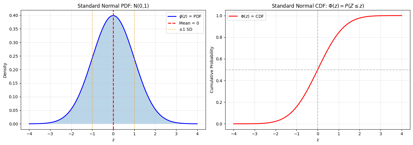
Standard Normal Properties:
P(Z ≤ 0) = 0.5000
P(-1 ≤ Z ≤ 1) = 0.6827
P(-2 ≤ Z ≤ 2) = 0.9545
P(-3 ≤ Z ≤ 3) = 0.9973
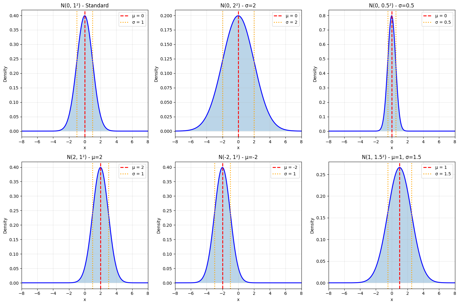
5.3.2 The Normal Distribution#
Now generalize to any mean \(\mu\) and variance \(\sigma^2\).
Definition 5.12: Normal Distribution#
A random variable \(X\) has a normal distribution with mean \(\mu\) and variance \(\sigma^2\) if:
for all \(x \in \mathbb{R}\).
We write \(X \sim N(\mu, \sigma^2)\) or \(X \sim \mathcal{N}(\mu, \sigma^2)\).
Note: Some sources use \(N(\mu, \sigma)\) (with standard deviation instead of variance). Always check!
Useful Facts 5.9: Mean and Variance of Normal#
For \(X \sim N(\mu, \sigma^2)\):
Mean: \(E[X] = \mu\)
Variance: \(\text{Var}(X) = \sigma^2\)
Standard deviation: \(\text{std}(X) = \sigma\)
Standardization#
Key Transformation: If \(X \sim N(\mu, \sigma^2)\), then:
This is called standardization or z-score transformation.
Reverse: If \(Z \sim N(0, 1)\), then:
Visualization of Different Parameters#
# Different normal distributions
params = [
    (0, 1, 'Standard'),
    (0, 2, 'σ=2'),
    (0, 0.5, 'σ=0.5'),
    (2, 1, 'μ=2'),
    (-2, 1, 'μ=-2'),
    (1, 1.5, 'μ=1, σ=1.5')
]

fig, axes = plt.subplots(2, 3, figsize=(15, 10))
axes = axes.flatten()

x = np.linspace(-8, 8, 1000)

for idx, (mu, sigma, desc) in enumerate(params):
    pdf = stats.norm.pdf(x, mu, sigma)

    axes[idx].plot(x, pdf, 'b-', linewidth=2)
    axes[idx].fill_between(x, 0, pdf, alpha=0.3)
    axes[idx].axvline(mu, color='r', linestyle='--', linewidth=2,
                      label=f'μ = {mu}')
    axes[idx].axvline(mu - sigma, color='orange', linestyle=':', linewidth=2)
    axes[idx].axvline(mu + sigma, color='orange', linestyle=':', linewidth=2,
                      label=f'σ = {sigma}')

    axes[idx].set_xlabel('x')
    axes[idx].set_ylabel('Density')
    axes[idx].set_title(f'N({mu}, {sigma}²) - {desc}')
    axes[idx].legend()
    axes[idx].grid(True, alpha=0.3)
    axes[idx].set_xlim([-8, 8])

plt.tight_layout()
plt.show()
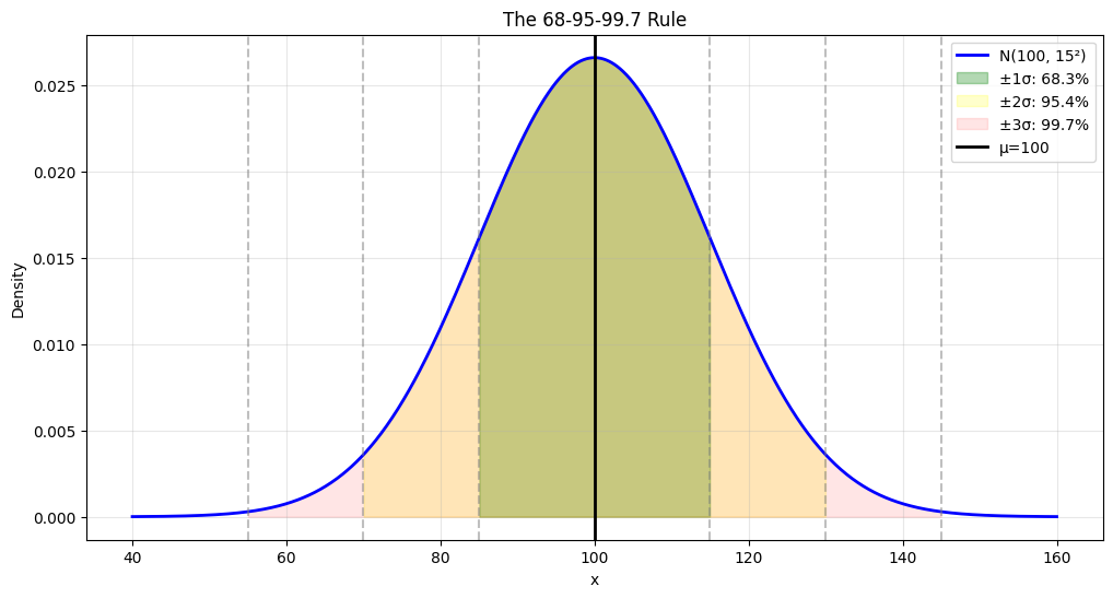
5.3.3 Properties of the Normal Distribution#
The 68-95-99.7 Rule (Empirical Rule)#
For \(X \sim N(\mu, \sigma^2)\):
68% of data within \(\mu \pm \sigma\)
95% of data within \(\mu \pm 2\sigma\)
99.7% of data within \(\mu \pm 3\sigma\)
# Visualize 68-95-99.7 rule
mu, sigma = 100, 15
x = np.linspace(mu - 4*sigma, mu + 4*sigma, 1000)
pdf = stats.norm.pdf(x, mu, sigma)

plt.figure(figsize=(12, 6))
plt.plot(x, pdf, 'b-', linewidth=2, label='N(100, 15²)')

# Fill regions
for k, color, alpha in [(1, 'green', 0.3), (2, 'yellow', 0.2), (3, 'red', 0.1)]:
    x_fill = x[(x >= mu - k*sigma) & (x <= mu + k*sigma)]
    pdf_fill = stats.norm.pdf(x_fill, mu, sigma)
    pct = stats.norm.cdf(mu + k*sigma, mu, sigma) - stats.norm.cdf(mu - k*sigma, mu, sigma)
    plt.fill_between(x_fill, 0, pdf_fill, alpha=alpha, color=color,
                     label=f'±{k}σ: {pct*100:.1f}%')

plt.axvline(mu, color='black', linestyle='-', linewidth=2, label=f'μ={mu}')
for k in [1, 2, 3]:
    plt.axvline(mu - k*sigma, color='gray', linestyle='--', alpha=0.5)
    plt.axvline(mu + k*sigma, color='gray', linestyle='--', alpha=0.5)

plt.xlabel('x')
plt.ylabel('Density')
plt.title('The 68-95-99.7 Rule')
plt.legend(loc='upper right')
plt.grid(True, alpha=0.3)
plt.show()
Linear Combinations#
Important Property: Normal distributions are closed under linear combinations.
If \(X \sim N(\mu_X, \sigma_X^2)\) and \(Y \sim N(\mu_Y, \sigma_Y^2)\) are independent, then:
Special case: If \(X_1, \ldots, X_n\) are independent \(N(\mu, \sigma^2)\), then:
# Demonstrate: Sum of normals is normal
np.random.seed(42)
mu1, sigma1 = 5, 2
mu2, sigma2 = 10, 3

# Theory
mu_sum = mu1 + mu2
sigma_sum = np.sqrt(sigma1**2 + sigma2**2)

# Simulation
n_sims = 100000
X = np.random.normal(mu1, sigma1, n_sims)
Y = np.random.normal(mu2, sigma2, n_sims)
S = X + Y

plt.figure(figsize=(12, 5))
plt.hist(S, bins=100, density=True, alpha=0.7, edgecolor='black',
         label='Simulated X + Y')

x = np.linspace(S.min(), S.max(), 1000)
plt.plot(x, stats.norm.pdf(x, mu_sum, sigma_sum), 'r-', linewidth=3,
         label=f'Theoretical N({mu_sum}, {sigma_sum**2:.1f})')

plt.xlabel('x')
plt.ylabel('Density')
plt.title(f'Sum of Normals: X~N({mu1},{sigma1}²) + Y~N({mu2},{sigma2}²)')
plt.legend()
plt.grid(True, alpha=0.3)
plt.show()

print(f"Theoretical: μ={mu_sum}, σ={sigma_sum:.3f}")
print(f"Simulated: μ={np.mean(S):.3f}, σ={np.std(S):.3f}")
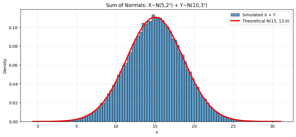
Theoretical: μ=15, σ=3.606
Simulated: μ=15.005, σ=3.614
Quantiles and Percentiles#
Definition: The \(p\)-quantile (or \(100p\)-th percentile) is the value \(x_p\) such that:
For standard normal \(Z \sim N(0,1)\):
\(z_{0.025} \approx -1.96\) (2.5th percentile)
\(z_{0.50} = 0\) (median)
\(z_{0.975} \approx 1.96\) (97.5th percentile)
# Important quantiles
quantiles = [0.01, 0.025, 0.05, 0.1, 0.5, 0.9, 0.95, 0.975, 0.99]

print("Standard Normal Quantiles:")
for q in quantiles:
    z_q = stats.norm.ppf(q, 0, 1)
    print(f"z_{{{q:.3f}}} = {z_q:6.3f}")

print("\nCommonly Used:")
print(f"z_0.025 = {stats.norm.ppf(0.025):.4f} (for 95% CI)")
print(f"z_0.005 = {stats.norm.ppf(0.005):.4f} (for 99% CI)")
Standard Normal Quantiles:
z_{0.010} = -2.326
z_{0.025} = -1.960
z_{0.050} = -1.645
z_{0.100} = -1.282
z_{0.500} =  0.000
z_{0.900} =  1.282
z_{0.950} =  1.645
z_{0.975} =  1.960
z_{0.990} =  2.326

Commonly Used:
z_0.025 = -1.9600 (for 95% CI)
z_0.005 = -2.5758 (for 99% CI)
Computing Probabilities#
Example: IQ scores are \(N(100, 15^2)\). What’s the probability someone has IQ > 130?
mu, sigma = 100, 15

# Method 1: Direct computation
prob1 = 1 - stats.norm.cdf(130, mu, sigma)

# Method 2: Standardize first
z = (130 - mu) / sigma
prob2 = 1 - stats.norm.cdf(z, 0, 1)

print(f"IQ scores: N({mu}, {sigma}²)")
print(f"P(IQ > 130) = {prob1:.4f}")
print(f"z-score of 130: {z:.2f}")
print(f"P(Z > {z:.2f}) = {prob2:.4f}")

# What IQ is at 95th percentile?
iq_95 = stats.norm.ppf(0.95, mu, sigma)
print(f"\n95th percentile IQ: {iq_95:.1f}")
IQ scores: N(100, 15²)
P(IQ > 130) = 0.0228
z-score of 130: 2.00
P(Z > 2.00) = 0.0228

95th percentile IQ: 124.7
The Central Limit Theorem (Informal)#
One of the most important theorems in all of probability!
Central Limit Theorem: The sum (or average) of many independent random variables approaches a normal distribution, regardless of the original distribution!
Demonstration#
# CLT demonstration with different source distributions
from scipy.stats import uniform, expon, beta as beta_dist

source_dists = [
    ('Uniform[0,1]', lambda n: np.random.uniform(0, 1, n)),
    ('Exponential(λ=1)', lambda n: np.random.exponential(1, n)),
    ('Beta(2,5)', lambda n: np.random.beta(2, 5, n)),
]

fig, axes = plt.subplots(len(source_dists), 4, figsize=(16, 12))

for row, (name, generator) in enumerate(source_dists):
    for col, n in enumerate([1, 5, 20, 50]):
        # Generate many sample means
        sample_means = [np.mean(generator(n)) for _ in range(10000)]

        ax = axes[row, col]
        ax.hist(sample_means, bins=50, density=True, alpha=0.7, edgecolor='black')

        # Overlay normal fit
        mu_hat = np.mean(sample_means)
        sigma_hat = np.std(sample_means)
        x = np.linspace(min(sample_means), max(sample_means), 100)
        ax.plot(x, stats.norm.pdf(x, mu_hat, sigma_hat), 'r-', linewidth=2,
                label='Normal fit')

        if col == 0:
            ax.set_ylabel(name, fontsize=11)
        if row == 0:
            ax.set_title(f'n = {n}', fontsize=11)
        if row == len(source_dists) - 1:
            ax.set_xlabel('Sample Mean')
        ax.legend(fontsize=8)
        ax.grid(True, alpha=0.3)

plt.suptitle('Central Limit Theorem: Distribution of Sample Means', fontsize=14, y=1.00)
plt.tight_layout()
plt.show()

print("Notice: As n increases, distribution approaches normal,")
print("        regardless of the source distribution!")
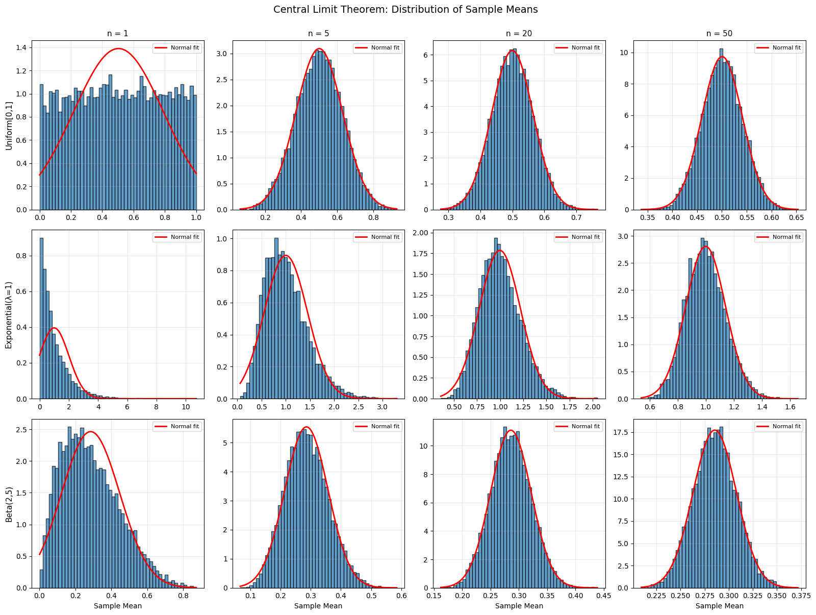
Notice: As n increases, distribution approaches normal,
        regardless of the source distribution!
Summary#
Key Facts About Normal Distribution
Standard Normal: \(Z \sim N(0, 1)\) $\(\phi(z) = \frac{1}{\sqrt{2\pi}} e^{-z^2/2}\)$
General Normal: \(X \sim N(\mu, \sigma^2)\) $\(p(x) = \frac{1}{\sigma\sqrt{2\pi}} e^{-(x-\mu)^2/(2\sigma^2)}\)$
Standardization: \(Z = \frac{X-\mu}{\sigma} \sim N(0,1)\)
68-95-99.7 Rule:
68% within \(\mu \pm \sigma\)
95% within \(\mu \pm 2\sigma\)
99.7% within \(\mu \pm 3\sigma\)
Linear combinations: \(aX + bY \sim N(a\mu_X + b\mu_Y, a^2\sigma_X^2 + b^2\sigma_Y^2)\)
Central Limit Theorem: Sample means → Normal
Practice Problems#
If \(X \sim N(50, 10^2)\), find:
\(P(X > 60)\)
\(P(40 < X < 55)\)
The 90th percentile of \(X\)
SAT scores are \(N(1000, 200^2)\). What percentage score above 1300?
If \(X \sim N(5, 4)\) and \(Y \sim N(3, 9)\) are independent, find the distribution of \(2X - Y + 1\).
Show that if \(X \sim N(\mu, \sigma^2)\), then \(aX + b \sim N(a\mu + b, a^2\sigma^2)\).
Use the CLT to explain why measurement errors are often normally distributed.
Next Section#
Now we’ll see how to approximate binomial distributions with normals when \(N\) is large!
→ Continue to 5.4 Normal Approximation to Binomial
→ Return to Chapter 5 Overview