![]()
6.2 Confidence Intervals#
A confidence interval provides a range of plausible values for a population parameter. It quantifies the uncertainty in our estimate.
The Big Idea#
Instead of saying “the population mean is exactly \((\bar{x})\)”, we say:
“We are 95% confident that the population mean lies between a and b”
This accounts for the fact that \((\bar{x})\) is based on a sample and has variability.
Constructing Confidence Intervals#
The General Form#
A confidence interval for a parameter θ has the form:
More precisely:
where:
\((\bar{x})\) is the sample mean (our estimate)
\((z_{\alpha/2})\) is a critical value from the standard normal distribution
\((\text{SE}(\bar{x}))\) is the standard error
Common Confidence Levels#
Confidence Level |
α |
zₐ/₂ |
|---|---|---|
90% |
0.10 |
1.645 |
95% |
0.05 |
1.960 |
99% |
0.01 |
2.576 |
Interpretation#
Correct: “If we repeated this sampling process many times and constructed a 95% CI each time, about 95% of those intervals would contain the true population mean μ.”
Incorrect: “There is a 95% probability that μ is in this specific interval.”
(Once the interval is computed, μ either is or isn’t in it - there’s no probability involved!)
Estimating the Standard Error#
The Problem#
The formula \((\text{SE}(\bar{X}) = \frac{\sigma}{\sqrt{n}})\) requires knowing σ, the population standard deviation. But usually we don’t know σ!
The Solution: Sample Standard Deviation#
We estimate σ using the sample standard deviation:
Note the \((n-1)\) in the denominator (Bessel’s correction) - this makes s an unbiased estimator of σ.
The t-Distribution#
When we replace σ with s, the distribution changes from normal to t-distribution:
where \((t_{n-1})\) is the t-distribution with \((n-1)\) degrees of freedom.
Properties of the t-distribution:
Symmetric and bell-shaped (like normal)
Heavier tails than normal (accounts for uncertainty in s)
As \((n \to \infty)\), \((t_{n-1} \to N(0,1))\)
Confidence Interval for Population Mean#
Case 1: Known Population Variance (σ² known)#
A \(((1-\alpha) \times 100\%)\) confidence interval for μ is:
Case 2: Unknown Population Variance (σ² unknown) - Most Common!#
A \(((1-\alpha) \times 100\%)\) confidence interval for μ is:
where \((t_{\alpha/2, n-1})\) is the critical value from the t-distribution with \((n-1)\) degrees of freedom.
Python Example: Computing Confidence Intervals#
import numpy as np
from scipy import stats
import matplotlib.pyplot as plt

def confidence_interval(data, confidence=0.95):
    """
    Compute confidence interval for population mean.

    Parameters:
    -----------
    data : array-like
        Sample data
    confidence : float
        Confidence level (default 0.95 for 95% CI)

    Returns:
    --------
    tuple : (lower_bound, upper_bound, margin_of_error)
    """
    n = len(data)
    mean = np.mean(data)
    se = stats.sem(data)  # Standard error of the mean

    # Degrees of freedom
    df = n - 1

    # t critical value
    alpha = 1 - confidence
    t_crit = stats.t.ppf(1 - alpha/2, df)

    # Margin of error
    margin = t_crit * se

    # Confidence interval
    ci_lower = mean - margin
    ci_upper = mean + margin

    return ci_lower, ci_upper, margin

# Example: Student test scores
np.random.seed(42)
scores = np.random.normal(75, 10, 30)  # 30 students, true mean=75, true std=10

# Compute 95% CI
lower, upper, margin = confidence_interval(scores, confidence=0.95)

print(f"Sample mean: {np.mean(scores):.2f}")
print(f"Sample std: {np.std(scores, ddof=1):.2f}")
print(f"Sample size: {len(scores)}")
print(f"\n95% Confidence Interval: [{lower:.2f}, {upper:.2f}]")
print(f"Margin of error: {margin:.2f}")
print(f"\nInterpretation: We are 95% confident that the true mean score")
print(f"is between {lower:.2f} and {upper:.2f}.")

# Compare with different confidence levels
print("\n" + "="*60)
print("Comparison of Different Confidence Levels")
print("="*60)
for conf in [0.90, 0.95, 0.99]:
    lower, upper, margin = confidence_interval(scores, confidence=conf)
    width = upper - lower
    print(f"{int(conf*100)}% CI: [{lower:6.2f}, {upper:6.2f}]  Width: {width:5.2f}  Margin: {margin:5.2f}")
Sample mean: 73.12
Sample std: 9.00
Sample size: 30

95% Confidence Interval: [69.76, 76.48]
Margin of error: 3.36

Interpretation: We are 95% confident that the true mean score
is between 69.76 and 76.48.

============================================================
Comparison of Different Confidence Levels
============================================================
90% CI: [ 70.33,  75.91]  Width:  5.58  Margin:  2.79
95% CI: [ 69.76,  76.48]  Width:  6.72  Margin:  3.36
99% CI: [ 68.59,  77.65]  Width:  9.06  Margin:  4.53
Observation: Higher confidence requires wider intervals!
Visualizing Confidence Intervals#
import numpy as np
import matplotlib.pyplot as plt
from scipy import stats

# True population
true_mean = 100
true_std = 15

# Function to generate CI from one sample
def generate_ci(sample_size=30, confidence=0.95):
    sample = np.random.normal(true_mean, true_std, sample_size)
    mean = np.mean(sample)
    se = stats.sem(sample)
    df = sample_size - 1
    alpha = 1 - confidence
    t_crit = stats.t.ppf(1 - alpha/2, df)
    margin = t_crit * se
    return mean, mean - margin, mean + margin

# Generate many CIs
np.random.seed(123)
n_intervals = 100
intervals = [generate_ci() for _ in range(n_intervals)]

# Check which intervals contain the true mean
contains_true = [lower <= true_mean <= upper for _, lower, upper in intervals]
n_contain = sum(contains_true)

# Plot
fig, ax = plt.subplots(figsize=(12, 10))

for i, (mean, lower, upper) in enumerate(intervals):
    color = 'green' if contains_true[i] else 'red'
    ax.plot([lower, upper], [i, i], color=color, linewidth=1, alpha=0.6)
    ax.plot(mean, i, 'o', color=color, markersize=3)

ax.axvline(true_mean, color='blue', linestyle='--', linewidth=2,
           label=f'True mean = {true_mean}')
ax.set_xlabel('Value', fontsize=12)
ax.set_ylabel('Sample Number', fontsize=12)
ax.set_title(f'100 × 95% Confidence Intervals\n{n_contain} contain the true mean (green), {n_intervals-n_contain} do not (red)',
             fontsize=14)
ax.legend(fontsize=11)
ax.grid(alpha=0.3, axis='x')

plt.tight_layout()
plt.savefig('confidence_intervals_simulation.png', dpi=150, bbox_inches='tight')
plt.show()

print(f"\nOut of {n_intervals} confidence intervals:")
print(f"  {n_contain} ({n_contain/n_intervals*100:.1f}%) contain the true mean")
print(f"  {n_intervals-n_contain} ({(n_intervals-n_contain)/n_intervals*100:.1f}%) do not")
print(f"\nExpected: ~95% should contain the true mean")
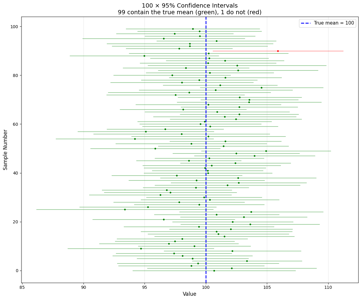
Out of 100 confidence intervals:
  99 (99.0%) contain the true mean
  1 (1.0%) do not

Expected: ~95% should contain the true mean
The Central Limit Theorem and CIs#
Why CIs Work#
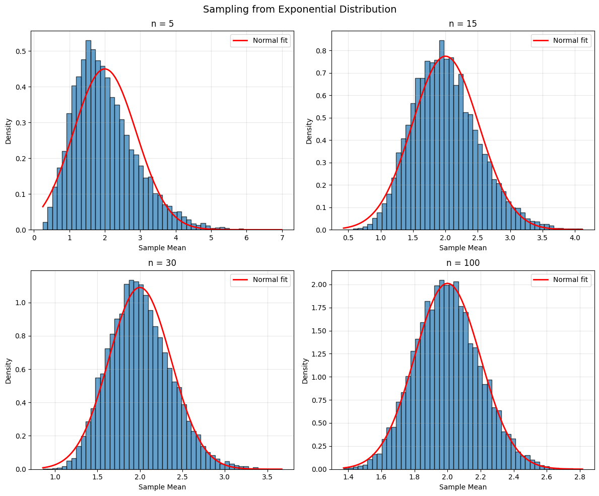
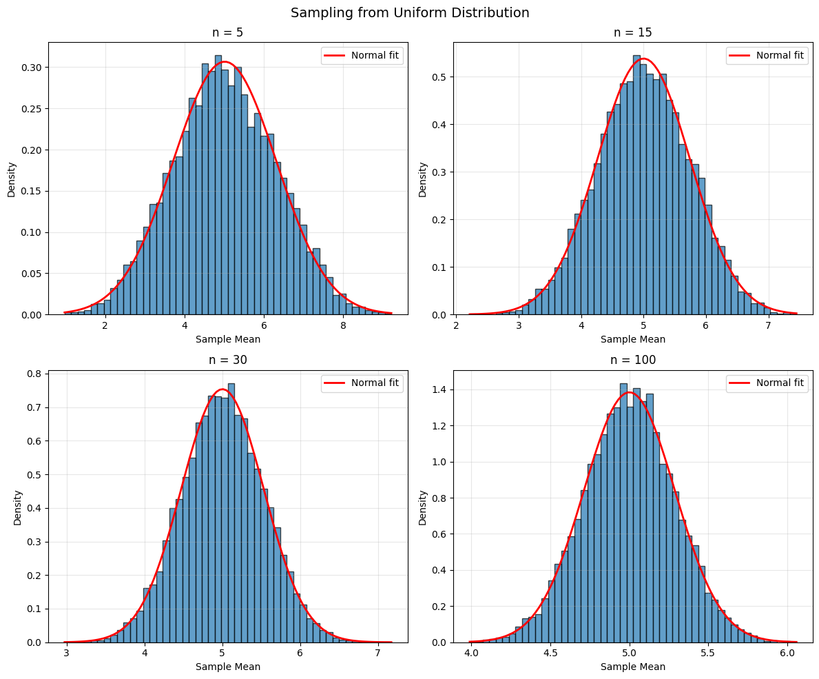
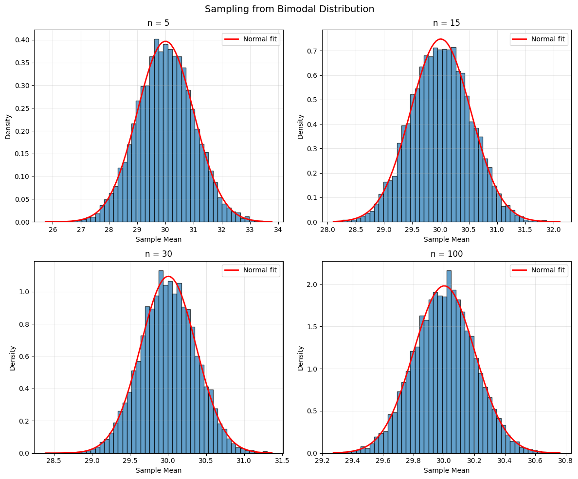
The Central Limit Theorem states that for large n:
approximately, regardless of the population distribution!
How Large is “Large Enough”?#
Symmetric, unimodal populations: n ≥ 15 is usually sufficient
Moderately skewed: n ≥ 30
Heavily skewed or extreme outliers: n ≥ 100 or more
Python Example: CLT in Action#
import numpy as np
import matplotlib.pyplot as plt
from scipy import stats

# Three very different populations
populations = {
    'Exponential': lambda n: np.random.exponential(2, n),
    'Uniform': lambda n: np.random.uniform(0, 10, n),
    'Bimodal': lambda n: np.concatenate([np.random.normal(20, 2, n//2),
                                          np.random.normal(40, 2, n//2)])
}

sample_sizes = [5, 15, 30, 100]

for pop_name, pop_func in populations.items():
    fig, axes = plt.subplots(2, 2, figsize=(12, 10))
    fig.suptitle(f'Sampling from {pop_name} Distribution', fontsize=14)
    axes = axes.ravel()

    for idx, n in enumerate(sample_sizes):
        # Generate many sample means
        sample_means = [np.mean(pop_func(n)) for _ in range(10000)]

        # Plot
        axes[idx].hist(sample_means, bins=50, density=True, alpha=0.7, edgecolor='black')

        # Overlay normal approximation
        mean_of_means = np.mean(sample_means)
        std_of_means = np.std(sample_means)
        x = np.linspace(min(sample_means), max(sample_means), 100)
        axes[idx].plot(x, stats.norm.pdf(x, mean_of_means, std_of_means),
                      'r-', linewidth=2, label='Normal fit')

        axes[idx].set_title(f'n = {n}')
        axes[idx].set_xlabel('Sample Mean')
        axes[idx].set_ylabel('Density')
        axes[idx].legend()
        axes[idx].grid(alpha=0.3)

    plt.tight_layout()
    plt.savefig(f'clt_{pop_name.lower()}.png', dpi=150, bbox_inches='tight')
    plt.show()
Standard Error from Simulation (Bootstrap)#
When the theoretical SE formula is complicated or unknown, we can estimate it via simulation:
The Bootstrap Method#
From the original sample of size n, draw many resamples (with replacement)
Compute the statistic of interest for each resample
The standard deviation of these statistics estimates the SE
import numpy as np
from scipy import stats

def bootstrap_ci(data, statistic=np.mean, n_bootstrap=10000, confidence=0.95):
    """
    Compute bootstrap confidence interval.

    Parameters:
    -----------
    data : array-like
        Original sample
    statistic : function
        Function to compute on each bootstrap sample (default: mean)
    n_bootstrap : int
        Number of bootstrap resamples
    confidence : float
        Confidence level

    Returns:
    --------
    tuple : (lower_bound, upper_bound, bootstrap_se)
    """
    n = len(data)
    bootstrap_stats = []

    for _ in range(n_bootstrap):
        # Resample with replacement
        resample = np.random.choice(data, size=n, replace=True)
        bootstrap_stats.append(statistic(resample))

    bootstrap_stats = np.array(bootstrap_stats)

    # Compute percentiles for CI
    alpha = 1 - confidence
    lower_percentile = (alpha/2) * 100
    upper_percentile = (1 - alpha/2) * 100

    ci_lower = np.percentile(bootstrap_stats, lower_percentile)
    ci_upper = np.percentile(bootstrap_stats, upper_percentile)

    # Bootstrap SE
    bootstrap_se = np.std(bootstrap_stats, ddof=1)

    return ci_lower, ci_upper, bootstrap_se

# Example
np.random.seed(42)
data = np.random.exponential(5, 50)  # Skewed data

print("Original sample:")
print(f"  Mean: {np.mean(data):.3f}")
print(f"  Median: {np.median(data):.3f}")
print(f"  n = {len(data)}")

# Bootstrap CI for mean
lower, upper, boot_se = bootstrap_ci(data, statistic=np.mean)
print(f"\nBootstrap 95% CI for mean: [{lower:.3f}, {upper:.3f}]")
print(f"Bootstrap SE: {boot_se:.3f}")

# Bootstrap CI for median
lower_med, upper_med, boot_se_med = bootstrap_ci(data, statistic=np.median)
print(f"\nBootstrap 95% CI for median: [{lower_med:.3f}, {upper_med:.3f}]")
print(f"Bootstrap SE: {boot_se_med:.3f}")

# Compare with traditional CI
traditional_lower, traditional_upper, _ = confidence_interval(data)
print(f"\nTraditional 95% CI for mean: [{traditional_lower:.3f}, {traditional_upper:.3f}]")
print(f"Traditional SE: {stats.sem(data):.3f}")
Original sample:
  Mean: 4.230
  Median: 2.864
  n = 50

Bootstrap 95% CI for mean: [3.057, 5.491]
Bootstrap SE: 0.621

Bootstrap 95% CI for median: [1.724, 4.133]
Bootstrap SE: 0.697

Traditional 95% CI for mean: [2.960, 5.500]
Traditional SE: 0.632
Practical Considerations#
Width of Confidence Intervals#
The width of a CI depends on:
Confidence level: Higher confidence → wider interval
Sample size: Larger n → narrower interval (by factor of (\sqrt{n}))
Population variability: Larger σ → wider interval
Common Mistakes#
❌ Wrong: “95% of the data falls in this interval” ✅ Right: “We’re 95% confident the population mean is in this interval”
❌ Wrong: “The probability that μ is in [a,b] is 0.95” ✅ Right: “If we repeated this process, 95% of intervals would contain μ”
❌ Wrong: Using z-values when σ is unknown ✅ Right: Using t-values when σ is estimated by s
Practice Problems#
Problem 1: Battery Life#
A sample of 16 batteries has mean lifetime 120 hours with standard deviation 15 hours. Construct a 95% confidence interval for the population mean.
Solution:
n = 16
mean = 120
s = 15
confidence = 0.95

# t critical value (df = 15)
t_crit = stats.t.ppf(0.975, df=15)  # 2.131
se = s / np.sqrt(n)  # 15/4 = 3.75
margin = t_crit * se  # 2.131 * 3.75 = 7.99

ci_lower = mean - margin  # 112.01
ci_upper = mean + margin  # 127.99

print(f"95% CI: [{ci_lower:.2f}, {ci_upper:.2f}]")
95% CI: [112.01, 127.99]
Answer: [112.01, 127.99] hours
Problem 2: Sample Size for Desired Margin#
You want a 95% CI for mean height with margin of error ± 2 cm. If σ = 10 cm, how large a sample do you need?
Solution: $\( E = z_{\alpha/2} \cdot \frac{\sigma}{\sqrt{n}} \implies 2 = 1.96 \cdot \frac{10}{\sqrt{n}} \)\( \)\( \sqrt{n} = \frac{1.96 \times 10}{2} = 9.8 \implies n = 96.04 \approx 97 \)$
Answer: Need n = 97 people
Problem 3: Interpreting Width#
Two 95% CIs are constructed: [45, 55] and [47, 53]. Which is based on a larger sample?
Solution: The second interval [47, 53] is narrower (width = 6 vs. 10), so it’s based on a larger sample.
Summary#
Key Formulas#
95% CI for population mean (σ unknown): $\( \bar{x} \pm t_{0.025, n-1} \cdot \frac{s}{\sqrt{n}} \)$
Sample size for desired margin E: $\( n = \left(\frac{z_{\alpha/2} \cdot \sigma}{E}\right)^2 \)$
Key Concepts#
Confidence intervals quantify uncertainty in estimates
Higher confidence requires wider intervals
Larger samples give narrower intervals (by (\sqrt{n}))
Use t-distribution when σ is unknown (almost always!)
Bootstrap provides CIs when formulas are unavailable
Correct interpretation is crucial - it’s about the process, not the specific interval
When to Use What#
Scenario |
Method |
|---|---|
σ known, any n |
z-interval |
σ unknown, large n (n ≥ 30) |
t-interval |
σ unknown, small n, normal pop |
t-interval |
Unknown distribution, any statistic |
Bootstrap |