![]()
9.2 Bayesian Inference#
The Bayesian Philosophy#
Bayesian inference treats parameters as random variables with probability distributions, unlike MLE which treats them as fixed unknown values.
Key Difference from MLE#
MLE (Frequentist): Parameter θ is fixed but unknown; estimate it from data
Bayesian: Parameter θ is a random variable; update beliefs about θ given data
Bayes’ Theorem for Parameters#
The Fundamental Formula#
Given data (x_1, \ldots, x_n) and parameter θ:
Components:
Posterior: (p(\theta \mid x_1, \ldots, x_n)) - Updated belief about θ after seeing data
Likelihood: (p(x_1, \ldots, x_n \mid \theta)) - Probability of data given θ
Prior: (p(\theta)) - Initial belief about θ before seeing data
Evidence: (p(x_1, \ldots, x_n)) - Marginal probability of data (normalizing constant)
Simplified Form#
Since the evidence is just a normalizing constant:
Or more intuitively:
Example 1: Coin Flipping (Beta-Binomial)#
Problem Setup#
Estimate probability (p) of heads from (n) coin flips with (k) heads observed.
Bayesian Solution#
Prior: Beta distribution (common choice for probabilities)
where (B(\alpha, \beta)) is the Beta function.
Likelihood: Binomial
Posterior: Also Beta! (conjugate prior)
Interpretation:
(\alpha) = prior “pseudo-counts” of heads
(\beta) = prior “pseudo-counts” of tails
Data adds (k) heads and (n-k) tails to these counts
Python Implementation#
import numpy as np
import matplotlib.pyplot as plt
from scipy import stats

np.random.seed(42)

# Generate data
true_p = 0.7
n_flips = 20
flips = np.random.binomial(1, true_p, n_flips)
k = np.sum(flips)

print("Bayesian Coin Flipping Example")
print("="*70)
print(f"True p: {true_p}")
print(f"Data: {k} heads in {n_flips} flips")
print()

# Different priors
priors = [
    (1, 1, "Uniform (uninformative)"),
    (2, 2, "Weak prior towards 0.5"),
    (10, 10, "Strong prior towards 0.5"),
    (5, 2, "Prior favoring heads")
]

p_range = np.linspace(0, 1, 1000)

fig, axes = plt.subplots(2, 2, figsize=(14, 10))
axes = axes.ravel()

for idx, (alpha, beta, label) in enumerate(priors):
    ax = axes[idx]

    # Prior distribution
    prior_dist = stats.beta(alpha, beta)
    prior_pdf = prior_dist.pdf(p_range)

    # Posterior distribution
    posterior_alpha = alpha + k
    posterior_beta = beta + (n_flips - k)
    posterior_dist = stats.beta(posterior_alpha, posterior_beta)
    posterior_pdf = posterior_dist.pdf(p_range)

    # Likelihood (normalized for plotting)
    likelihood = p_range**k * (1-p_range)**(n_flips-k)
    likelihood = likelihood / np.max(likelihood) * np.max(posterior_pdf)

    # Plot
    ax.plot(p_range, prior_pdf, 'b--', linewidth=2, label='Prior', alpha=0.7)
    ax.plot(p_range, likelihood, 'g:', linewidth=2, label='Likelihood (scaled)', alpha=0.7)
    ax.plot(p_range, posterior_pdf, 'r-', linewidth=2.5, label='Posterior')
    ax.axvline(true_p, color='black', linestyle='--', linewidth=1.5,
               label=f'True p = {true_p}', alpha=0.5)

    # MLE for comparison
    p_mle = k / n_flips
    ax.axvline(p_mle, color='orange', linestyle='--', linewidth=1.5,
               label=f'MLE = {p_mle:.2f}', alpha=0.7)

    # Posterior mean
    post_mean = posterior_alpha / (posterior_alpha + posterior_beta)
    ax.axvline(post_mean, color='red', linestyle=':', linewidth=1.5,
               label=f'Posterior mean = {post_mean:.2f}', alpha=0.7)

    ax.set_xlabel('p (probability of heads)', fontsize=11)
    ax.set_ylabel('Density', fontsize=11)
    ax.set_title(f'{label}\nBeta({alpha}, {beta}) → Beta({posterior_alpha}, {posterior_beta})',
                 fontsize=12)
    ax.legend(fontsize=9, loc='upper left')
    ax.grid(alpha=0.3)
    ax.set_xlim(0, 1)

plt.tight_layout()
plt.savefig('bayesian_coin_priors.png', dpi=150, bbox_inches='tight')
plt.show()

print("\nPosterior Statistics:")
for alpha, beta, label in priors:
    post_alpha = alpha + k
    post_beta = beta + (n_flips - k)
    post_mean = post_alpha / (post_alpha + post_beta)
    post_mode = (post_alpha - 1) / (post_alpha + post_beta - 2)
    post_var = (post_alpha * post_beta) / ((post_alpha + post_beta)**2 * (post_alpha + post_beta + 1))

    print(f"\n{label}:")
    print(f"  Posterior: Beta({post_alpha}, {post_beta})")
    print(f"  Mean: {post_mean:.3f}")
    print(f"  Mode: {post_mode:.3f}")
    print(f"  Std: {np.sqrt(post_var):.3f}")
Bayesian Coin Flipping Example
======================================================================
True p: 0.7
Data: 14 heads in 20 flips
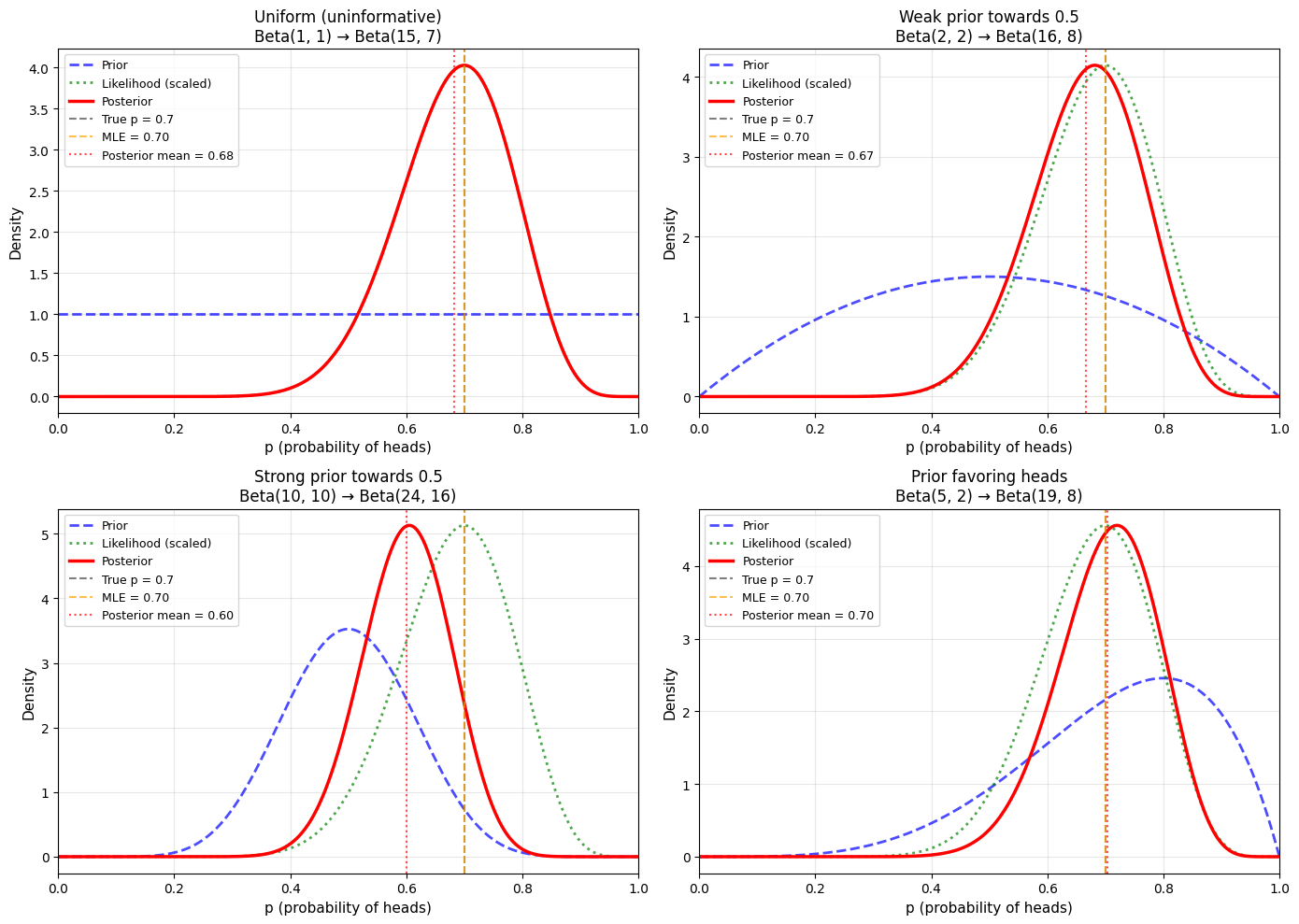
Posterior Statistics:

Uniform (uninformative):
  Posterior: Beta(15, 7)
  Mean: 0.682
  Mode: 0.700
  Std: 0.097

Weak prior towards 0.5:
  Posterior: Beta(16, 8)
  Mean: 0.667
  Mode: 0.682
  Std: 0.094

Strong prior towards 0.5:
  Posterior: Beta(24, 16)
  Mean: 0.600
  Mode: 0.605
  Std: 0.077

Prior favoring heads:
  Posterior: Beta(19, 8)
  Mean: 0.704
  Mode: 0.720
  Std: 0.086
Credible Intervals#
Definition#
A 95% credible interval ([a, b]) satisfies:
Interpretation: “There is a 95% probability that θ lies in ([a, b]) given the data we observed.”
Credible Intervals vs. Confidence Intervals#
Credible Interval (Bayesian):
Direct probability statement about the parameter
“θ has 95% probability of being in this interval”
Confidence Interval (Frequentist):
Statement about the procedure, not the parameter
“If we repeat this procedure many times, 95% of intervals will contain the true θ”
Computing Credible Intervals#
import numpy as np
from scipy import stats

# Continuing from previous example
alpha, beta = 1, 1  # Uniform prior
k, n_flips = 14, 20  # Observed data

# Posterior
post_alpha = alpha + k
post_beta = beta + (n_flips - k)
posterior = stats.beta(post_alpha, post_beta)

print("Credible Intervals")
print("="*70)

# Equal-tailed 95% credible interval
lower = posterior.ppf(0.025)
upper = posterior.ppf(0.975)
print(f"\n95% Equal-tailed credible interval: [{lower:.3f}, {upper:.3f}]")

# Highest Posterior Density (HPD) interval
# For unimodal symmetric distributions, similar to equal-tailed
print(f"\nInterpretation: Given the data, there is a 95% probability")
print(f"that the true probability of heads is between {lower:.3f} and {upper:.3f}")

# Compare with frequentist confidence interval
p_mle = k / n_flips
se = np.sqrt(p_mle * (1 - p_mle) / n_flips)
ci_lower = p_mle - 1.96 * se
ci_upper = p_mle + 1.96 * se

print(f"\n95% Frequentist confidence interval: [{ci_lower:.3f}, {ci_upper:.3f}]")
print(f"\nNote: These are often numerically similar but have different interpretations!")
Credible Intervals
======================================================================

95% Equal-tailed credible interval: [0.478, 0.854]

Interpretation: Given the data, there is a 95% probability
that the true probability of heads is between 0.478 and 0.854

95% Frequentist confidence interval: [0.499, 0.901]

Note: These are often numerically similar but have different interpretations!
Prior Selection#
Types of Priors#
1. Informative Prior: Incorporates specific prior knowledge
2. Weakly Informative Prior: General shape but not too strong
3. Non-informative (Uniform) Prior: No prior knowledge
Choosing Priors#
Guidelines:
Use domain knowledge when available
Check sensitivity: Try different priors, see if conclusions change
With large data, prior becomes less important
Document your choice and reasoning
Sequential Updating#
Bayesian Learning#
One beautiful property: today’s posterior = tomorrow’s prior
Example: Sequential Coin Flips#
import numpy as np
import matplotlib.pyplot as plt
from scipy import stats

np.random.seed(42)

# True parameter
true_p = 0.6

# Start with uniform prior
alpha, beta = 1, 1

# Generate data in batches
batch_sizes = [5, 10, 20, 50]
p_range = np.linspace(0, 1, 1000)

fig, axes = plt.subplots(2, 2, figsize=(14, 10))
axes = axes.ravel()

for idx, n_new in enumerate(batch_sizes):
    # Generate new data
    new_flips = np.random.binomial(1, true_p, n_new)
    k_new = np.sum(new_flips)

    # Update posterior
    alpha += k_new
    beta += (n_new - k_new)

    # Current posterior
    posterior = stats.beta(alpha, beta)

    ax = axes[idx]
    ax.plot(p_range, posterior.pdf(p_range), 'b-', linewidth=2.5,
            label=f'Posterior: Beta({alpha}, {beta})')
    ax.axvline(true_p, color='red', linestyle='--', linewidth=2,
               label=f'True p = {true_p}')

    post_mean = alpha / (alpha + beta)
    ax.axvline(post_mean, color='green', linestyle=':', linewidth=2,
               label=f'Posterior mean = {post_mean:.3f}')

    ax.fill_between(p_range, posterior.pdf(p_range), alpha=0.3)

    total_flips = alpha + beta - 2  # Subtract initial prior counts
    ax.set_xlabel('p', fontsize=11)
    ax.set_ylabel('Posterior Density', fontsize=11)
    ax.set_title(f'After {total_flips} total flips ({k_new} heads in last {n_new})',
                 fontsize=12)
    ax.legend(fontsize=10)
    ax.grid(alpha=0.3)
    ax.set_xlim(0, 1)

plt.tight_layout()
plt.savefig('sequential_updating.png', dpi=150, bbox_inches='tight')
plt.show()

print("\nSequential Bayesian Updating")
print("="*70)
print(f"Final posterior after all data: Beta({alpha}, {beta})")
print(f"Posterior mean: {alpha / (alpha + beta):.3f}")
print(f"True p: {true_p}")
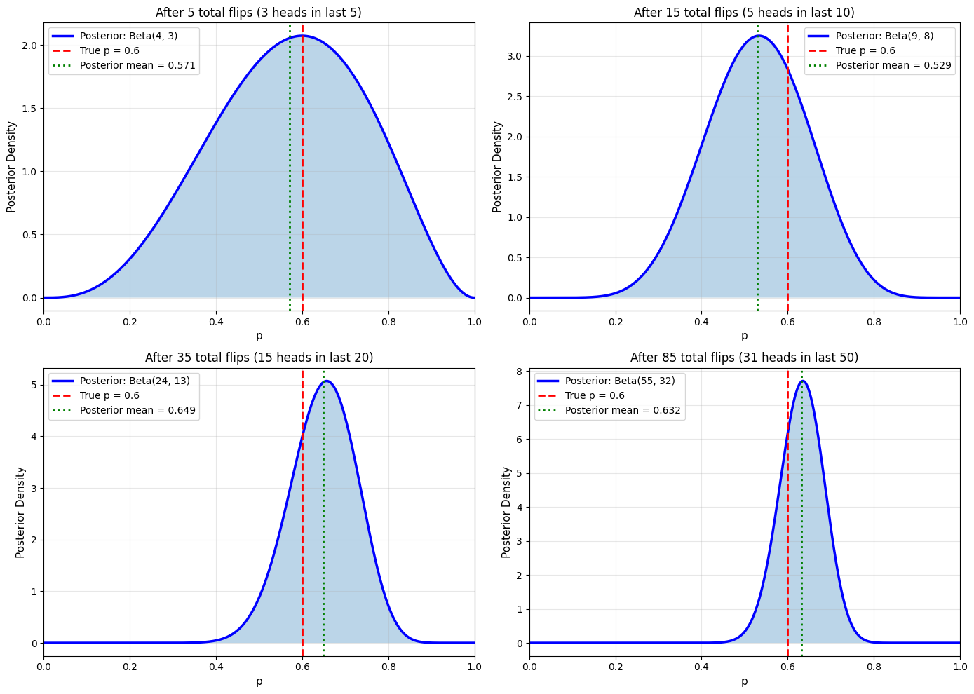
Sequential Bayesian Updating
======================================================================
Final posterior after all data: Beta(55, 32)
Posterior mean: 0.632
True p: 0.6
Posterior Predictive Distribution#
Definition#
Predict new data (\tilde{x}) given observed data:
Interpretation: Average predictions over all possible parameter values, weighted by their posterior probability.
Example: Predicting Next Coin Flip#
import numpy as np
from scipy import stats

# Observed data: 7 heads in 10 flips
alpha_prior, beta_prior = 1, 1
k, n = 7, 10

# Posterior
alpha_post = alpha_prior + k
beta_post = beta_prior + (n - k)

print("Posterior Predictive Distribution")
print("="*70)
print(f"\nObserved: {k} heads in {n} flips")
print(f"Posterior: Beta({alpha_post}, {beta_post})")
print()

# Probability that next flip is heads
# For Beta-Binomial, this has a closed form:
prob_heads = alpha_post / (alpha_post + beta_post)

print(f"Predicted probability of heads on next flip: {prob_heads:.3f}")
print(f"\n(Compare to MLE: {k/n:.3f})")
print(f"\nNote: Bayesian prediction accounts for uncertainty in p!")
Posterior Predictive Distribution
======================================================================

Observed: 7 heads in 10 flips
Posterior: Beta(8, 4)

Predicted probability of heads on next flip: 0.667

(Compare to MLE: 0.700)

Note: Bayesian prediction accounts for uncertainty in p!
Summary#
Key Concepts#
Bayes’ Theorem:
Posterior ∝ Likelihood × Prior
Advantages of Bayesian Inference#
✅ Incorporates prior knowledge ✅ Provides full distribution over parameters ✅ Natural sequential updating ✅ Direct probability statements ✅ Automatic regularization (via prior)
Challenges#
❌ Requires prior specification ❌ Computational complexity (often needs MCMC) ❌ Sensitive to prior with small data ❌ More conceptually complex
When to Use Bayesian vs. MLE#
Use Bayesian when:
You have good prior information
You want uncertainty quantification
Small sample sizes
Sequential learning is important
Use MLE when:
Large sample sizes
No prior information
Computational simplicity needed
Standard errors are sufficient