![]()
8.2 Two-Factor Experiments: Two-Way ANOVA#
Beyond One Factor#
The Limitation of One-Way ANOVA#
One-way ANOVA studies one factor at a time:
Different fertilizers
Different teaching methods
Different drug dosages
But real-world outcomes often depend on multiple factors!
Two-Way ANOVA#
Studies two factors simultaneously:
Fertilizer type and watering schedule
Teaching method and class size
Drug dosage and patient age
Advantages#
More efficient: Study two factors in one experiment
Detect interactions: See if factors work together
More realistic: Real systems have multiple influences
The Two-Way ANOVA Model#
Notation#
Factor A has a levels (e.g., 3 fertilizer types)
Factor B has b levels (e.g., 2 watering schedules)
n replicates per combination (cell)
Total observations: N = a × b × n
The Model#
where:
(\mu) = grand mean
(\alpha_i) = effect of level i of Factor A
(\beta_j) = effect of level j of Factor B
((\alpha\beta)_{ij}) = interaction effect
(\epsilon_{ijk}) = random error
Three Hypotheses#
Main Effect of Factor A:
H₀ᴬ: (\alpha_1 = \alpha_2 = \cdots = \alpha_a = 0) (no effect of A)
H₁ᴬ: At least one (\alpha_i \neq 0)
Main Effect of Factor B:
H₀ᴮ: (\beta_1 = \beta_2 = \cdots = \beta_b = 0) (no effect of B)
H₁ᴮ: At least one (\beta_j \neq 0)
Interaction A×B:
H₀ᴬᴮ: ((\alpha\beta)_{ij} = 0) for all i, j (no interaction)
H₁ᴬᴮ: At least one ((\alpha\beta)_{ij} \neq 0)
Understanding Interactions#
What is an Interaction?#
An interaction occurs when the effect of one factor depends on the level of another factor.
Example: No Interaction#
Fertilizer effect is the same regardless of watering:
   Yield
     ^
  30 |
     |     B (high water)
  25 |    /
     |   /
  20 |  /  A (low water)
     | /
  15 |/
     +----------> Fertilizer
        1   2   3

Parallel lines = No interaction
Example: Interaction Present#
Fertilizer effect depends on watering:

   Yield
     ^
  30 |        B (high water)
     |       /
  25 |      /
     |     X
  20 |    /  \
     |   /    \ A (low water)
  15 |  /      \
     +----------> Fertilizer
        1   2   3

Crossing lines = Interaction!
Partitioning Variance in Two-Way ANOVA#
Sum of Squares Decomposition#
where:
SST: Total sum of squares
SSA: Sum of squares for Factor A
SSB: Sum of squares for Factor B
SSAB: Sum of squares for interaction A×B
SSE: Sum of squares for error (residual)
Degrees of Freedom#
dfₐ: a - 1 (Factor A)
dfᴮ: b - 1 (Factor B)
dfₐᴮ: (a-1)(b-1) (Interaction)
dfₑ: ab(n-1) (Error)
dfₜ: abn - 1 (Total)
F-Statistics#
Python Example: Fertilizer × Watering#
import numpy as np
import pandas as pd
from scipy import stats
import matplotlib.pyplot as plt
import seaborn as sns
np.random.seed(42)
# Create experimental data
# Factor A: Fertilizer (3 types)
# Factor B: Water (2 levels: low, high)
# n = 5 replicates per cell
data = {
'Yield': [
# Fertilizer 1, Low water
18, 19, 17, 20, 18,
# Fertilizer 1, High water
22, 24, 23, 25, 23,
# Fertilizer 2, Low water
20, 21, 19, 22, 21,
# Fertilizer 2, High water
28, 30, 29, 31, 29,
# Fertilizer 3, Low water
17, 18, 16, 19, 17,
# Fertilizer 3, High water
20, 21, 19, 22, 21
],
'Fertilizer': ['F1']*10 + ['F2']*10 + ['F3']*10,
'Water': ['Low']*5 + ['High']*5 + ['Low']*5 + ['High']*5 + ['Low']*5 + ['High']*5
}
df = pd.DataFrame(data)
print("Two-Way ANOVA: Fertilizer × Watering")
print("="*70)
print("\nData Summary:")
print(df.groupby(['Fertilizer', 'Water'])['Yield'].agg(['mean', 'std', 'count']))
# Perform two-way ANOVA using statsmodels
try:
from statsmodels.formula.api import ols
from statsmodels.stats.anova import anova_lm
# Fit the model
model = ols('Yield ~ C(Fertilizer) + C(Water) + C(Fertilizer):C(Water)', data=df).fit()
# ANOVA table
anova_table = anova_lm(model, typ=2)
print("\n" + "="*70)
print("ANOVA Table")
print("="*70)
print(anova_table)
# Extract p-values
p_fertilizer = anova_table.loc['C(Fertilizer)', 'PR(>F)']
p_water = anova_table.loc['C(Water)', 'PR(>F)']
p_interaction = anova_table.loc['C(Fertilizer):C(Water)', 'PR(>F)']
print("\n" + "="*70)
print("Interpretation")
print("="*70)
alpha = 0.05
print(f"\nMain Effect of Fertilizer: p = {p_fertilizer:.4f}")
if p_fertilizer < alpha:
print(" → Significant: Fertilizer type affects yield")
else:
print(" → Not significant: No effect of fertilizer type")
print(f"\nMain Effect of Water: p = {p_water:.4f}")
if p_water < alpha:
print(" → Significant: Watering level affects yield")
else:
print(" → Not significant: No effect of watering level")
print(f"\nInteraction Fertilizer × Water: p = {p_interaction:.4f}")
if p_interaction < alpha:
print(" → Significant: Effect of fertilizer depends on watering!")
print(" Must interpret main effects carefully.")
else:
print(" → Not significant: Fertilizer and water act independently")
print(" Main effects can be interpreted separately.")
except ImportError:
print("\nPlease install statsmodels: pip install statsmodels")
print("Performing manual calculation...")
# Manual calculation (simplified)
grand_mean = df['Yield'].mean()
# Cell means
cell_means = df.groupby(['Fertilizer', 'Water'])['Yield'].mean()
print(f"\nCell means:\n{cell_means}")
# Visualization
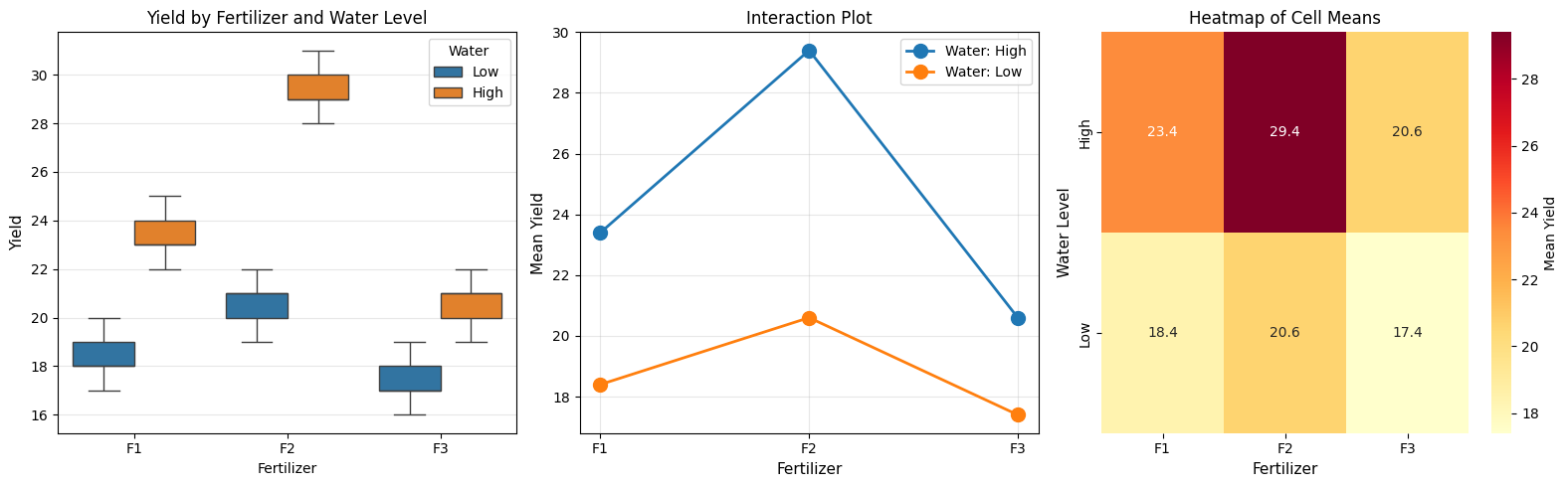
fig, axes = plt.subplots(1, 3, figsize=(16, 5))
# 1. Box plot by both factors
sns.boxplot(data=df, x='Fertilizer', y='Yield', hue='Water', ax=axes[0])
axes[0].set_title('Yield by Fertilizer and Water Level', fontsize=12)
axes[0].set_ylabel('Yield', fontsize=11)
axes[0].legend(title='Water')
axes[0].grid(alpha=0.3, axis='y')
# 2. Interaction plot
means = df.groupby(['Fertilizer', 'Water'])['Yield'].mean().unstack()
for water_level in means.columns:
axes[1].plot(means.index, means[water_level], 'o-',
linewidth=2, markersize=10, label=f'Water: {water_level}')
axes[1].set_xlabel('Fertilizer', fontsize=11)
axes[1].set_ylabel('Mean Yield', fontsize=11)
axes[1].set_title('Interaction Plot', fontsize=12)
axes[1].legend()
axes[1].grid(alpha=0.3)
# 3. Heatmap of cell means
cell_means_pivot = df.groupby(['Water', 'Fertilizer'])['Yield'].mean().unstack()
sns.heatmap(cell_means_pivot, annot=True, fmt='.1f', cmap='YlOrRd',
ax=axes[2], cbar_kws={'label': 'Mean Yield'})
axes[2].set_title('Heatmap of Cell Means', fontsize=12)
axes[2].set_ylabel('Water Level', fontsize=11)
axes[2].set_xlabel('Fertilizer', fontsize=11)
plt.tight_layout()
plt.savefig('two_way_anova.png', dpi=150, bbox_inches='tight')
plt.show()
Two-Way ANOVA: Fertilizer × Watering
======================================================================

Data Summary:
                  mean       std  count
Fertilizer Water
F1         High   23.4  1.140175      5
           Low    18.4  1.140175      5
F2         High   29.4  1.140175      5
           Low    20.6  1.140175      5
F3         High   20.6  1.140175      5
           Low    17.4  1.140175      5

======================================================================
ANOVA Table
======================================================================
                            sum_sq    df           F        PR(>F)
C(Fertilizer)           188.066667   2.0   72.333333  6.889437e-11
C(Water)                240.833333   1.0  185.256410  8.831093e-13
C(Fertilizer):C(Water)   40.866667   2.0   15.717949  4.335527e-05
Residual                 31.200000  24.0         NaN           NaN

======================================================================
Interpretation
======================================================================

Main Effect of Fertilizer: p = 0.0000
  → Significant: Fertilizer type affects yield

Main Effect of Water: p = 0.0000
  → Significant: Watering level affects yield

Interaction Fertilizer × Water: p = 0.0000
  → Significant: Effect of fertilizer depends on watering!
     Must interpret main effects carefully.
Interpreting Interactions#
Rule of Thumb#
Always test interaction first
If interaction is significant:
Main effects may be misleading
Describe the interaction pattern
Consider simple effects analysis
If no interaction:
Interpret main effects independently
Simple Effects Analysis#
When interaction is significant, test effects of one factor at each level of the other.
def simple_effects_analysis(df, factor1, factor2, response):
    """
    Analyze simple effects when interaction is significant.
    """
    print(f"Simple Effects: {factor1} at each level of {factor2}")
    print("="*70)

    for level in df[factor2].unique():
        subset = df[df[factor2] == level]
        groups = [subset[subset[factor1] == f][response].values
                  for f in subset[factor1].unique()]

        f_stat, p_value = stats.f_oneway(*groups)

        print(f"\n{factor2} = {level}:")
        print(f"  F-statistic = {f_stat:.3f}")
        print(f"  p-value = {p_value:.4f}")
        if p_value < 0.05:
            print(f"  → {factor1} has significant effect at {factor2} = {level}")
        else:
            print(f"  → {factor1} has no significant effect at {factor2} = {level}")

# Example usage
if p_interaction < 0.05:
    simple_effects_analysis(df, 'Fertilizer', 'Water', 'Yield')
Simple Effects: Fertilizer at each level of Water
======================================================================

Water = Low:
  F-statistic = 10.308
  p-value = 0.0025
  → Fertilizer has significant effect at Water = Low

Water = High:
  F-statistic = 77.744
  p-value = 0.0000
  → Fertilizer has significant effect at Water = High
Balanced vs. Unbalanced Designs#
Balanced Design#
Equal sample sizes in all cells (nᵢⱼ = n for all i,j)
Advantages:
Simpler calculations
More robust to assumption violations
Equal power for all tests
Unbalanced Design#
Unequal sample sizes across cells
Challenges:
Different sum of squares types (Type I, II, III)
Interpretation more complex
Less robust
Recommendation: Always strive for balanced designs!
Effect Sizes in Two-Way ANOVA#
Partial Eta-Squared#
Proportion of variance explained by each factor, controlling for other factors:
def partial_eta_squared(anova_table):
    """
    Calculate partial eta-squared for each effect.
    """
    print("\nEffect Sizes (Partial η²)")
    print("="*60)

    SSE = anova_table.loc['Residual', 'sum_sq']

    for index in anova_table.index[:-1]:  # Exclude residual
        SS_effect = anova_table.loc[index, 'sum_sq']
        eta_sq_p = SS_effect / (SS_effect + SSE)

        if eta_sq_p < 0.01:
            size = "negligible"
        elif eta_sq_p < 0.06:
            size = "small"
        elif eta_sq_p < 0.14:
            size = "medium"
        else:
            size = "large"

        print(f"{index:<30}: η²_p = {eta_sq_p:.3f} ({size})")

partial_eta_squared(anova_table)
Effect Sizes (Partial η²)
============================================================
C(Fertilizer)                 : η²_p = 0.858 (large)
C(Water)                      : η²_p = 0.885 (large)
C(Fertilizer):C(Water)        : η²_p = 0.567 (large)
Assumptions of Two-Way ANOVA#
Same as one-way ANOVA:
Independence of observations
Normality within each cell
Homogeneity of variance across all cells
Checking Assumptions#
def check_two_way_assumptions(df, factor1, factor2, response):
    """
    Check ANOVA assumptions for two-way design.
    """
    # 1. Homogeneity of variance (Levene's test)
    groups = [df[(df[factor1]==f1) & (df[factor2]==f2)][response].values
              for f1 in df[factor1].unique()
              for f2 in df[factor2].unique()]

    stat, p = stats.levene(*groups)
    print("Homogeneity of Variance (Levene's Test)")
    print(f"  Statistic = {stat:.3f}, p-value = {p:.4f}")
    if p > 0.05:
        print("  → Assumption satisfied (p > 0.05)")
    else:
        print("  → WARNING: Variances may be unequal (p < 0.05)")

    # 2. Normality (residuals)
    try:
        from statsmodels.formula.api import ols
        model = ols(f'{response} ~ C({factor1}) + C({factor2}) + C({factor1}):C({factor2})',
                    data=df).fit()
        residuals = model.resid

        stat, p = stats.shapiro(residuals)
        print("\nNormality of Residuals (Shapiro-Wilk Test)")
        print(f"  Statistic = {stat:.3f}, p-value = {p:.4f}")
        if p > 0.05:
            print("  → Assumption satisfied (p > 0.05)")
        else:
            print("  → WARNING: Residuals may not be normal (p < 0.05)")
    except:
        print("\nInstall statsmodels to check normality of residuals")

check_two_way_assumptions(df, 'Fertilizer', 'Water', 'Yield')
Homogeneity of Variance (Levene's Test)
  Statistic = 0.000, p-value = 1.0000
  → Assumption satisfied (p > 0.05)

Normality of Residuals (Shapiro-Wilk Test)
  Statistic = 0.915, p-value = 0.0199
  → WARNING: Residuals may not be normal (p < 0.05)
Summary#
When to Use Two-Way ANOVA#
✅ Two categorical independent variables (factors)
✅ One continuous dependent variable
✅ Want to study main effects AND interactions
✅ Balanced design (equal n per cell) preferred
Key Concepts#
Main effects: Effect of each factor averaged over the other
Interaction: Effect of one factor depends on the other
Test interaction first: Guides interpretation of main effects
Balanced designs: Simplify analysis and interpretation
Effect sizes: Report partial η² for each effect
Two-Way ANOVA Table Template#
Source |
SS |
df |
MS |
F |
p-value |
|---|---|---|---|---|---|
Factor A |
SSA |
a-1 |
MSA |
Fₐ |
pₐ |
Factor B |
SSB |
b-1 |
MSB |
Fᴮ |
pᴮ |
A × B |
SSAB |
(a-1)(b-1) |
MSAB |
Fₐᴮ |
pₐᴮ |
Error |
SSE |
ab(n-1) |
MSE |
||
Total |
SST |
abn-1 |