![]()
5.1 Discrete Distributions#
Most random phenomena we encounter fall into a small number of standard patterns. Discrete distributions model situations where outcomes take on distinct, countable values like integers.
5.1.1 The Discrete Uniform Distribution#
The simplest discrete distribution: all outcomes are equally likely.
Definition 5.1: Uniform Random Variable (Discrete)#
A random variable has the discrete uniform distribution if it takes each of \(k\) values with the same probability \(\frac{1}{k}\), and all other values with probability zero.
Examples#
import numpy as np
import matplotlib.pyplot as plt
from scipy import stats

# Example 1: Fair die
values_die = np.arange(1, 7)
probs_die = np.ones(6) / 6

# Example 2: Card ranks (1-52)
values_card = np.arange(1, 53)
probs_card = np.ones(52) / 52

# Visualize
fig, axes = plt.subplots(1, 2, figsize=(14, 5))

axes[0].bar(values_die, probs_die, edgecolor='black', alpha=0.7)
axes[0].set_xlabel('Die Face')
axes[0].set_ylabel('Probability')
axes[0].set_title('Discrete Uniform: Fair Die')
axes[0].set_xticks(values_die)
axes[0].grid(True, alpha=0.3, axis='y')

axes[1].bar(values_card[:13], probs_card[:13], edgecolor='black', alpha=0.7)
axes[1].set_xlabel('Card Value (showing first 13)')
axes[1].set_ylabel('Probability')
axes[1].set_title('Discrete Uniform: Card Deck (first suit)')
axes[1].grid(True, alpha=0.3, axis='y')

plt.tight_layout()
plt.show()

print("Fair Die:")
print(f"  Each value: {probs_die[0]:.4f} probability")
print(f"  Mean: {np.sum(values_die * probs_die):.2f}")
print(f"\nCard Deck (all 52):")
print(f"  Each value: {probs_card[0]:.4f} probability")
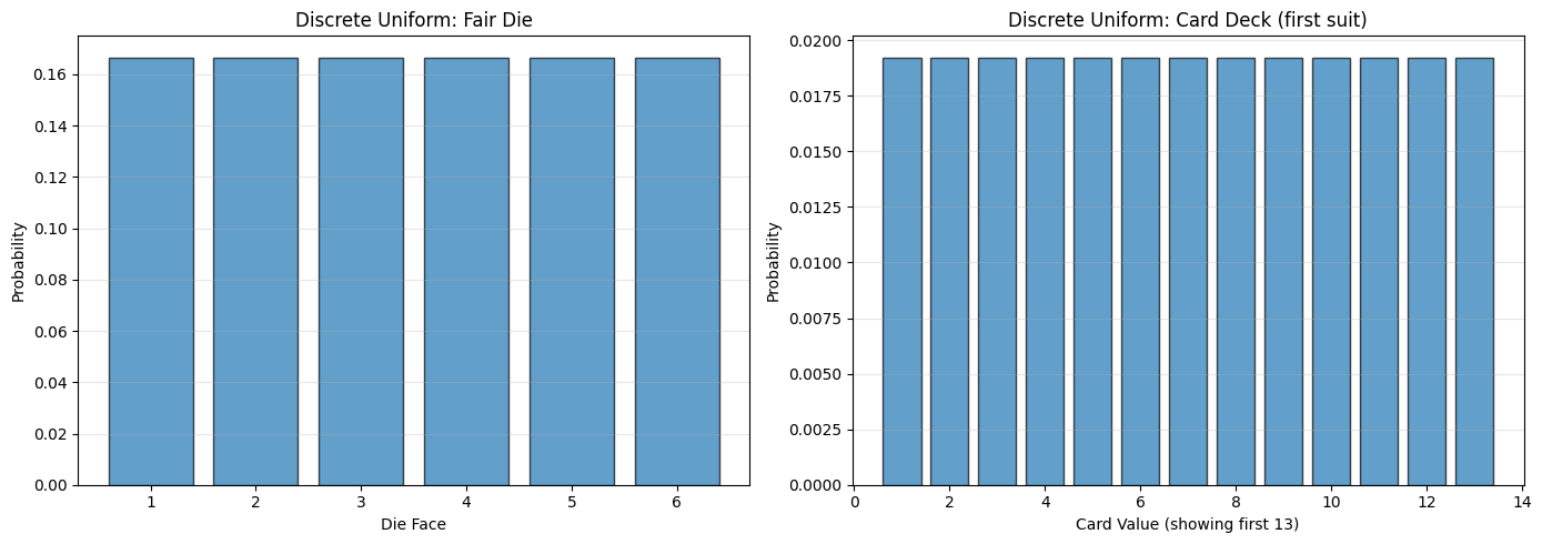
Fair Die:
  Each value: 0.1667 probability
  Mean: 3.50

Card Deck (all 52):
  Each value: 0.0192 probability
Important Note: If two random variables have a uniform distribution, their sum and difference will NOT be uniform! (See Chapter 4, Example 4.3)
5.1.2 Bernoulli Random Variables#
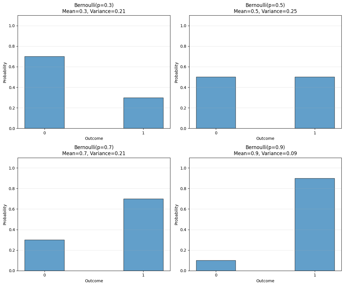
A Bernoulli random variable models a single trial with two outcomes: success (1) or failure (0).
Definition 5.2: Bernoulli Random Variable#
A Bernoulli random variable takes the value \(1\) with probability \(p\) and \(0\) with probability \(1-p\).
This is a model for:
A coin toss (heads/tails)
A test result (pass/fail)
A click (yes/no)
Any binary outcome
Useful Facts 5.1: Mean and Variance of Bernoulli#
A Bernoulli random variable with parameter \(p\) has:
Mean: \(p\)
Variance: \(p(1-p)\)
Derivation#
# Bernoulli demonstrations
p_values = [0.3, 0.5, 0.7, 0.9]

fig, axes = plt.subplots(2, 2, figsize=(12, 10))
axes = axes.flatten()

for idx, p in enumerate(p_values):
    # PMF
    values = [0, 1]
    probs = [1-p, p]

    axes[idx].bar(values, probs, width=0.4, edgecolor='black', alpha=0.7)
    axes[idx].set_xlabel('Outcome')
    axes[idx].set_ylabel('Probability')
    axes[idx].set_title(f'Bernoulli(p={p})\nMean={p:.1f}, Variance={p*(1-p):.2f}')
    axes[idx].set_xticks([0, 1])
    axes[idx].set_ylim([0, 1.1])
    axes[idx].grid(True, alpha=0.3, axis='y')

plt.tight_layout()
plt.show()
5.1.3 The Geometric Distribution#
Question: How many trials until the first success?
Motivation#
You flip a biased coin with \(P(H) = p\) until the first head appears. How many flips did it take?
To get exactly \(n\) flips: need \((n-1)\) tails then 1 head
Probability: \((1-p)^{n-1} \cdot p\)
Definition 5.3: Geometric Distribution#
The geometric distribution is a probability distribution on positive integers \(n \geq 1\):
where \(0 < p \leq 1\) is called the parameter of the distribution.
Useful Facts 5.2: Mean and Variance of Geometric#
A geometric distribution with parameter \(p\) has:
Mean: \(\frac{1}{p}\)
Variance: \(\frac{1-p}{p^2}\)
Examples and Interpretation#
# Geometric distributions
from scipy.stats import geom

p_values = [0.1, 0.3, 0.5, 0.7]
fig, axes = plt.subplots(2, 2, figsize=(14, 10))
axes = axes.flatten()

for idx, p in enumerate(p_values):
    n = np.arange(1, 21)
    probs = geom.pmf(n, p)

    mean = 1/p
    var = (1-p)/(p**2)

    axes[idx].bar(n, probs, edgecolor='black', alpha=0.7)
    axes[idx].axvline(mean, color='r', linestyle='--', linewidth=2,
                      label=f'Mean = {mean:.2f}')
    axes[idx].set_xlabel('Number of Trials')
    axes[idx].set_ylabel('Probability')
    axes[idx].set_title(f'Geometric(p={p})\nMean={mean:.2f}, Std={np.sqrt(var):.2f}')
    axes[idx].legend()
    axes[idx].grid(True, alpha=0.3, axis='y')

plt.tight_layout()
plt.show()

print("Interpretation:")
for p in [0.1, 0.5, 0.9]:
    mean = 1/p
    print(f"p={p}: Average {mean:.1f} trials until first success")
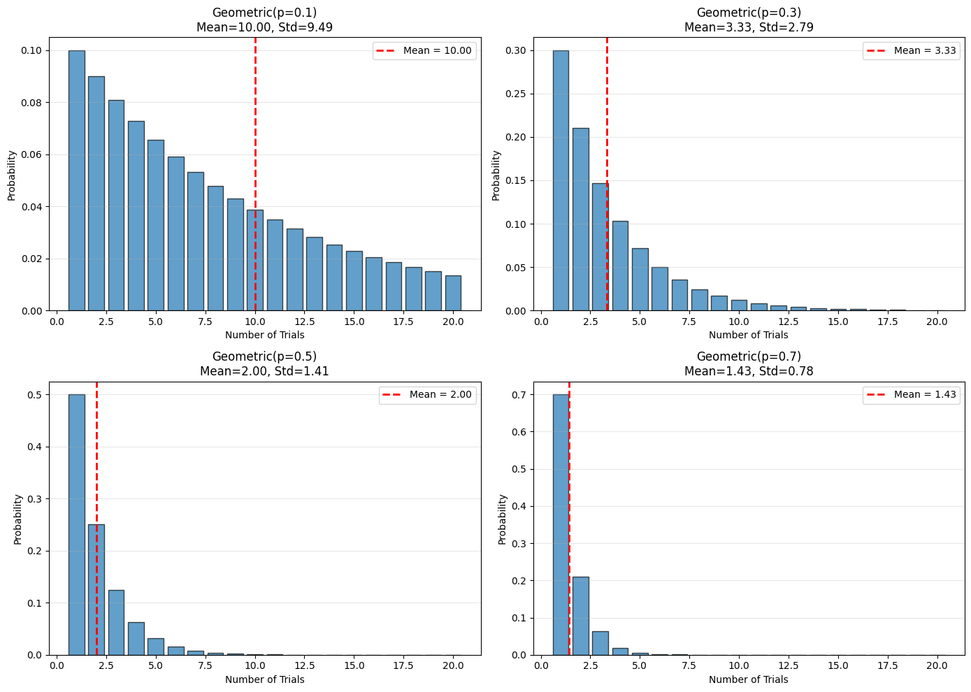
Interpretation:
p=0.1: Average 10.0 trials until first success
p=0.5: Average 2.0 trials until first success
p=0.9: Average 1.1 trials until first success
Key Insight: The geometric distribution models waiting times for first success.
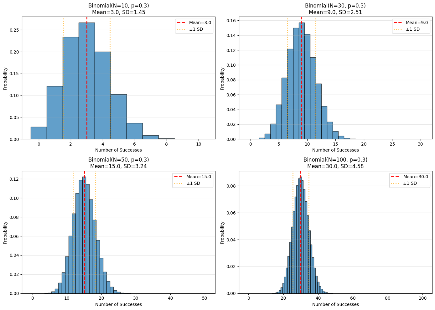
5.1.4 The Binomial Distribution#
Question: How many successes in \(N\) trials?
Motivation#
Flip a biased coin \(N\) times. How many times does it come up heads?
Number of ways to get \(h\) heads in \(N\) flips: \(\binom{N}{h}\)
Probability of each specific sequence with \(h\) heads: \(p^h(1-p)^{N-h}\)
Definition 5.4: Binomial Distribution#
In \(N\) independent repetitions of an experiment with binary outcome:
for \(0 \leq h \leq N\), and \(P_b(h; N, p) = 0\) otherwise.
Useful Facts 5.3: Mean and Variance of Binomial#
The binomial distribution \(P_b(h; N, p)\) has:
Mean: \(Np\)
Variance: \(Np(1-p)\)
Proof (Important!)#
Proposition: The mean of \(P_b(h; N, p)\) is \(Np\). The variance is \(Np(1-p)\).
Proof: Write \(X\) for a random variable with distribution \(P_b(h; N, p)\).
Notice that \(X\) can be written as sum of Bernoulli variables:
$\(X = Y_1 + Y_2 + \cdots + Y_N\)$
where \(Y_i = 1\) if the \(i\)-th trial is a success, 0 otherwise.
By linearity of expectation:
$\(E[X] = E[Y_1 + \cdots + Y_N] = E[Y_1] + \cdots + E[Y_N] = Np\)$
Since the trials are independent:
$\(\text{Var}(X) = \text{Var}(Y_1) + \cdots + \text{Var}(Y_N) = Np(1-p)\)$
Visualization#
# Binomial distributions
from scipy.stats import binom

fig, axes = plt.subplots(2, 2, figsize=(14, 10))

# Fix p, vary N
p = 0.3
for idx, N in enumerate([10, 30, 50, 100]):
    ax = axes[idx // 2, idx % 2]
    h = np.arange(0, N+1)
    probs = binom.pmf(h, N, p)

    mean = N * p
    std = np.sqrt(N * p * (1-p))

    ax.bar(h, probs, edgecolor='black', alpha=0.7, width=1)
    ax.axvline(mean, color='r', linestyle='--', linewidth=2, label=f'Mean={mean:.1f}')
    ax.axvline(mean - std, color='orange', linestyle=':', linewidth=2, alpha=0.7)
    ax.axvline(mean + std, color='orange', linestyle=':', linewidth=2, alpha=0.7,
               label=f'±1 SD')

    ax.set_xlabel('Number of Successes')
    ax.set_ylabel('Probability')
    ax.set_title(f'Binomial(N={N}, p={p})\nMean={mean:.1f}, SD={std:.2f}')
    ax.legend()
    ax.grid(True, alpha=0.3, axis='y')

plt.tight_layout()
plt.show()
Properties#
Recurrence relation: $\(P_b(h; N, p) = p \cdot P_b(h-1; N-1, p) + (1-p) \cdot P_b(h; N-1, p)\)$
Symmetry: $\(P_b(N-i; N, p) = P_b(i; N, 1-p)\)$
5.1.5 Multinomial Probabilities#
Generalization: What if there are more than 2 outcomes?
Definition 5.5: Multinomial Distribution#
Perform \(N\) independent repetitions of an experiment with \(k\) possible outcomes. The \(i\)-th outcome has probability \(p_i\).
The probability of observing outcome 1 exactly \(n_1\) times, outcome 2 exactly \(n_2\) times, …, outcome \(k\) exactly \(n_k\) times (where \(n_1 + n_2 + \cdots + n_k = N\)) is:
Example: Die Rolls#
from scipy.stats import multinomial

# Roll a fair die 10 times
N = 10
probs = [1/6] * 6  # Fair die

# What's the probability of getting exactly [2,2,2,2,1,1]?
outcome = [2, 2, 2, 2, 1, 1]
prob = multinomial.pmf(outcome, N, probs)

print(f"Rolling a die {N} times:")
print(f"Probability of outcome {outcome}: {prob:.6f}")

# Simulate to verify
np.random.seed(42)
num_sims = 100000
count = 0

for _ in range(num_sims):
    rolls = np.random.choice(range(1, 7), size=N, p=probs)
    counts = [np.sum(rolls == i) for i in range(1, 7)]
    if counts == outcome:
        count += 1

empirical_prob = count / num_sims
print(f"Simulated probability: {empirical_prob:.6f}")
Rolling a die 10 times:
Probability of outcome [2, 2, 2, 2, 1, 1]: 0.003751
Simulated probability: 0.003700
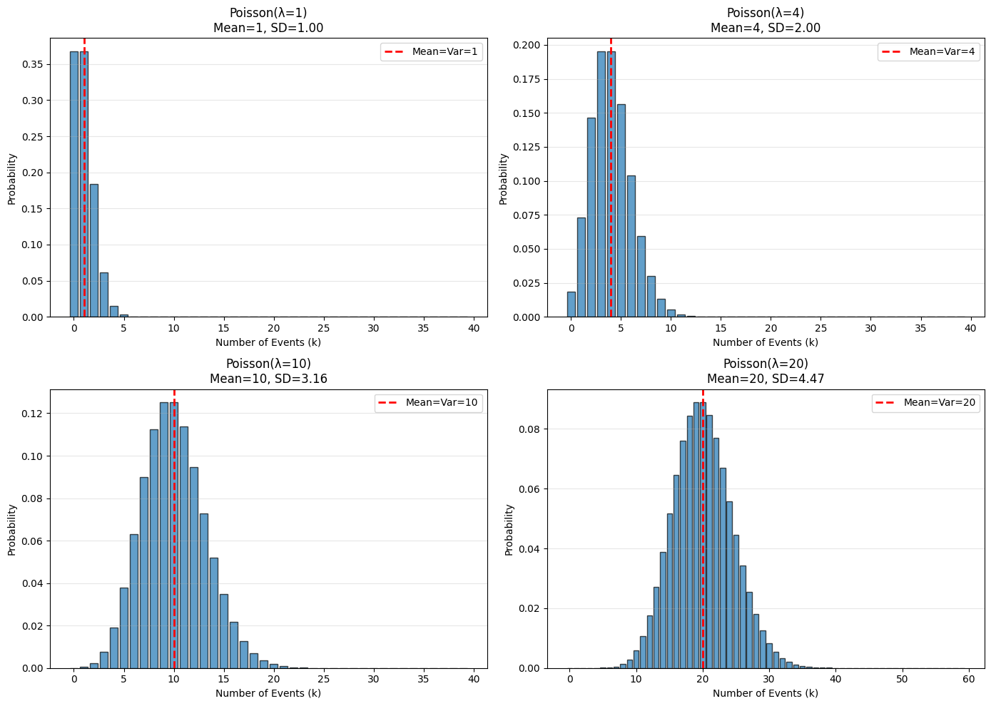
5.1.6 The Poisson Distribution#
Models: Counts of rare events occurring at a constant average rate.
When to Use Poisson#
Two key properties:
Events occur at some fixed average rate
Occurrence is independent of time since last event
Definition 5.6: Poisson Distribution#
A non-negative, integer-valued random variable \(X\) has a Poisson distribution when:
where \(\lambda > 0\) is the intensity parameter.
Useful Facts 5.4: Mean and Variance of Poisson#
A Poisson distribution with intensity \(\lambda\) has:
Mean: \(\lambda\)
Variance: \(\lambda\)
Yes, they’re the same!
Classic Examples#
Number of calls to a call center per minute
Number of Prussian soldiers killed by horse-kicks per year
Number of typos per page
Number of insurance claims per month
Number of emails received per hour
Visualization#
from scipy.stats import poisson

lambdas = [1, 4, 10, 20]
fig, axes = plt.subplots(2, 2, figsize=(14, 10))
axes = axes.flatten()

for idx, lam in enumerate(lambdas):
    k = np.arange(0, max(40, int(lam * 3)))
    probs = poisson.pmf(k, lam)

    axes[idx].bar(k, probs, edgecolor='black', alpha=0.7)
    axes[idx].axvline(lam, color='r', linestyle='--', linewidth=2,
                      label=f'Mean=Var={lam}')
    axes[idx].set_xlabel('Number of Events (k)')
    axes[idx].set_ylabel('Probability')
    axes[idx].set_title(f'Poisson(λ={lam})\nMean={lam}, SD={np.sqrt(lam):.2f}')
    axes[idx].legend()
    axes[idx].grid(True, alpha=0.3, axis='y')

plt.tight_layout()
plt.show()
Poisson Point Process#
Spatial Generalization: A Poisson point process with intensity \(\lambda\) has:
Number of points in an interval of length \(s\): Poisson(\(\lambda s\))
Number of points in an area \(A\): Poisson(\(\lambda \cdot \text{area}(A)\))
Applications:
Roadkill locations on a highway
Positions of trees in a forest
Stars in the sky
Customer arrivals at a store
# Simulate Poisson point process in 2D
np.random.seed(42)
lambda_intensity = 100  # points per unit area
area = 1.0  # 1x1 square

# Number of points is Poisson(λ * area)
num_points = np.random.poisson(lambda_intensity * area)

# Positions are uniform in the area
x = np.random.uniform(0, 1, num_points)
y = np.random.uniform(0, 1, num_points)

plt.figure(figsize=(8, 8))
plt.scatter(x, y, alpha=0.6, s=20)
plt.xlabel('x')
plt.ylabel('y')
plt.title(f'Poisson Point Process\nλ={lambda_intensity}, Generated {num_points} points')
plt.grid(True, alpha=0.3)
plt.axis('equal')
plt.show()

print(f"Expected number of points: {lambda_intensity * area}")
print(f"Actually generated: {num_points}")
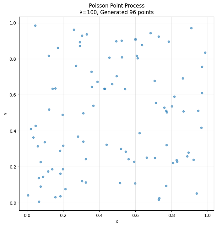
Expected number of points: 100.0
Actually generated: 96
Summary Table#
Distribution |
PMF |
Mean |
Variance |
Used For |
|---|---|---|---|---|
Discrete Uniform |
\(\frac{1}{k}\) |
\(\frac{k+1}{2}\) (if 1 to k) |
varies |
Equal probabilities |
Bernoulli |
\(p^x(1-p)^{1-x}\) |
\(p\) |
\(p(1-p)\) |
Single trial |
Geometric |
\((1-p)^{n-1}p\) |
\(\frac{1}{p}\) |
\(\frac{1-p}{p^2}\) |
Trials until success |
Binomial |
\(\binom{N}{k}p^k(1-p)^{N-k}\) |
\(Np\) |
\(Np(1-p)\) |
Successes in N trials |
Multinomial |
\(\frac{N!}{n_1!\cdots n_k!}p_1^{n_1}\cdots p_k^{n_k}\) |
varies |
varies |
Multiple outcomes |
Poisson |
\(\frac{\lambda^k e^{-\lambda}}{k!}\) |
\(\lambda\) |
\(\lambda\) |
Rare event counts |
Practice Problems#
You flip a coin with \(P(H) = 0.3\) ten times. What’s the probability of:
Exactly 3 heads?
At least 5 heads?
The first head appears on the 4th flip?
A call center receives an average of 5 calls per minute. What’s the probability of:
Receiving exactly 3 calls in the next minute?
Receiving 10 or more calls in the next minute?
Receiving no calls in the next minute?
Show that the Poisson distribution sums to 1: \(\sum_{k=0}^{\infty} \frac{\lambda^k e^{-\lambda}}{k!} = 1\)
A die is rolled until a 6 appears. What’s the expected number of rolls?
Next Section#
Now we’ll explore continuous probability distributions!
→ Continue to 5.2 Continuous Distributions
→ Return to Chapter 5 Overview