This page continues directly from Uninformed Search — Theory and Algorithms, which covers state-space representation and blind search strategies (BFS, DFS, UCS, Bidirectional Search).
2.3 Informed Search Algorithms¶
Informed search uses problem-specific knowledge through heuristic functions to guide search more efficiently toward goals.
Heuristic Function h(n)¶
Definition: Estimated cost from node n to the nearest goal.
Example (8-puzzle):
h(n) = number of misplaced tiles
h(n) = sum of Manhattan distances of tiles
Key Properties:
Admissible: Never overestimates true cost
h(n) ≤ h*(n) where h*(n) is true cost to goalConsistent (Monotonic): Satisfies triangle inequality
h(n) ≤ c(n,n’) + h(n’) for every edge (n,n’)
Evaluation Functions¶
g(n): Actual cost from start to n
h(n): Estimated cost from n to goal
f(n): Total estimated cost of solution through n
2.3.1 Best-First Search (Greedy Search)¶
Evaluation Function: f(n) = h(n)
Strategy: Expand node that appears closest to goal based on heuristic estimate.
How it works:
Maintain priority queue ordered by h(n)
Always expand node with smallest h(n)
Ignore cost to reach current node
Best-First Search (Greedy Search) VS The Uniform Cost Search¶
Using UCS (actual costs only):
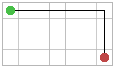
The node c is a dead end. The next node with the lowest cost is d (3), so it is selected for expansion next.
Using Best-First Search (heuristic only): an estimation of the cost from each node to the goal node G is provided by a heuristic function h(n).
A Heuristic Function h(n) is used to estimate the cost from node n to the goal node G. It could be:
The straight-line distance between two cities in a route-finding problem.
The Manhattan distance in a grid-based pathfinding problem.
The number of misplaced tiles in the 8-puzzle problem.


2.3.2 A* Search¶
A* is the most widely used informed search algorithm, combining actual and estimated costs.
Evaluation Function:
Where:
g(n): Actual cost from start to n
h(n): Estimated cost from n to goal
f(n): Estimated total cost of solution through n
Algorithm GenericSearch(Initial State: s, Goal Condition: G)
 begin
	LIST= { s };
	repeat
		Select current node i from LIST based on pre-defined strategy;
		Delete node i from LIST;
		Add node i to the hash table VISIT;
		for all nodes j ∈ A(i) directly connected to i via transition do
		begin
			if (j is not in VISIT) add j to LIST;
			pred(j)=i;
			choose the node j according to f(j):
				f(j) = min{c(j)} // Uniform Cost Search
				f(j) = min{h(j)} // Best-First Search
				f(j) = min{c(j) + h(j)} // A* Search
		end
	until LIST is empty or current node i satisfies G;
	if current node satisfies G return success
		else return failure;
	{ The predecessor array can be used to trace back path from i to s }
 end
How it works:
Maintain priority queue ordered by f(n) = g(n) + h(n)
Always expand node with smallest f(n)
Balance between:
Nodes close to start (small g)
Nodes close to goal (small h)
Why A* is Optimal¶
Theorem: If h(n) is admissible, A* finds the optimal solution.
Proof Sketch:
Suppose A* returns suboptimal goal G₂ with cost C₂
Let G be optimal goal with cost C* < C₂
Some unexpanded node n must be on optimal path to G
Since h is admissible:
f(n) = g(n) + h(n) ≤ g(n) + h*(n) = C*
Therefore: f(n) ≤ C* < C₂ = f(G₂)
But A* expands nodes in order of f-value
So n would be expanded before G₂
Contradiction! ∎
When Should A* Terminate?¶
A* should terminate when the goal node is selected for expansion from the list. This ensures the path found is optimal.
Example demonstrating why:
| Step | Node | f = g + h | Result |
|---|---|---|---|
| 1 | S | 0 + 3 = 3 | Expand, add a(f=4), b(f=3) |
| 2 | b | 2 + 1 = 3 | Expand, add G(f=5) via b |
| 3 | a | 2 + 2 = 4 | Expand, add G(f=4) via a |
| 4 | G | 4 + 0 = 4 | Goal selected for expansion → terminate! |
Optimal path: S → a → G (cost = 4), not S → b → G (cost = 5)
Is A* Always Optimal?¶
A* is optimal only if the heuristic is admissible:
Admissible: h(n) never overestimates the true cost to reach the goal.
For every node n: h(n) ≤ h*(n) where h*(n) is the actual cost to goal.
Counter-example with inadmissible heuristic:
h(S) = 7 (but true cost is 4 via S→a→G) — Overestimates!
A* explores: S(f=7) → a(f=7) → but G via S has f=5, so A* might return cost=5 instead of optimal cost=4
2.3.3 Designing Heuristics¶
Good heuristics make search efficient. Here are examples for common problems.
Example 1: 8-Puzzle¶
Problem: Slide tiles to reach goal configuration.
Heuristic 1: Misplaced Tiles
Admissible? Yes (each misplaced tile requires ≥1 move)
Quality: Moderate
Heuristic 2: Manhattan Distance
Admissible? Yes (tiles can’t jump, need ≥ Manhattan distance moves)
Quality: Better than h₁
Example State:
Current:        Goal:
1 2 3           1 2 3
4 5 6           4 5 6
7   8           7 8

h₁ = 1 (tile 8 misplaced)
h₂ = 1 (tile 8 needs 1 move)
Empirical Results:
| Heuristic | Avg Nodes Expanded |
|---|---|
| None (UCS) | ~170,000 |
| Misplaced (h₁) | ~500 |
| Manhattan (h₂) | ~50 |
Techniques for Creating Heuristics¶
1. Relaxed Problem
Remove constraints from original problem:
8-puzzle: Allow tiles to move anywhere → Manhattan distance
Route planning: Ignore roads → straight-line distance
2. Pattern Databases
Precompute optimal costs for subproblems:
8-puzzle: Store costs for positioning each tile
Rubik’s cube: Store costs for corner positions
3. Learning
Train a function to estimate costs:
Use neural network
Learn from experience
Properties of Good Heuristics¶
✓ Admissible: Guarantees optimality
✓ Consistent: Enables efficient search
✓ Accurate: Close to true cost (but never over)
✓ Fast to compute: Overhead shouldn’t exceed savings
2.4 Local Search Algorithms¶
Local search algorithms focus on exploring the immediate neighborhood of the current solution to find an improved solution. Unlike global search algorithms that explore the entire search space:
They don’t track paths taken
They only care about final state quality
They use state-centric loss functions
They make incremental changes to iteratively refine solutions
Applications:
Scheduling problems
Circuit design
Eight-queens (complete-state approach)
Traveling salesperson problem
VLSI layout
Vehicle routing
2.4.1 Hill Climbing¶
Hill climbing is a greedy local search algorithm that iteratively moves towards the neighbor state with the lowest loss (or highest value) until no better neighbors are found.
Algorithm:
Algorithm: HillClimbing(Initial State s, Loss Function L)
begin
    current ← s
    loop
        neighbors ← generate_neighbors(current)
        if neighbors is empty then
            return current

        next ← neighbor with minimum L(neighbor)

        if L(next) ≥ L(current) then
            return current  // Local optimum

        current ← next
end
Hill Climbing Example 1: Eight-Queens¶
Solving the 8-queens problem using Hill Climbing:
Start with a random configuration of 8 queens on the chessboard
Evaluate the number of pairs of queens attacking each other (the loss function)
Move a queen to a different position in its column to reduce attacking pairs
Repeat until zero attacking pairs (success) or no improvement possible (stuck)
State: 8 queens on board (may attack each other)
Neighbor: Move one queen to different row in same column
Loss: Number of pairs of queens attacking each other
Goal: Loss = 0
Hill Climbing Example 2: Traveling Salesperson¶
Solving TSP using Hill Climbing:
Start with a random tour of all cities
Evaluate the total distance of the tour (loss function)
Swap positions of two cities in the tour to reduce total distance
Repeat until no swap improves the tour
The Problem of Local Optima¶
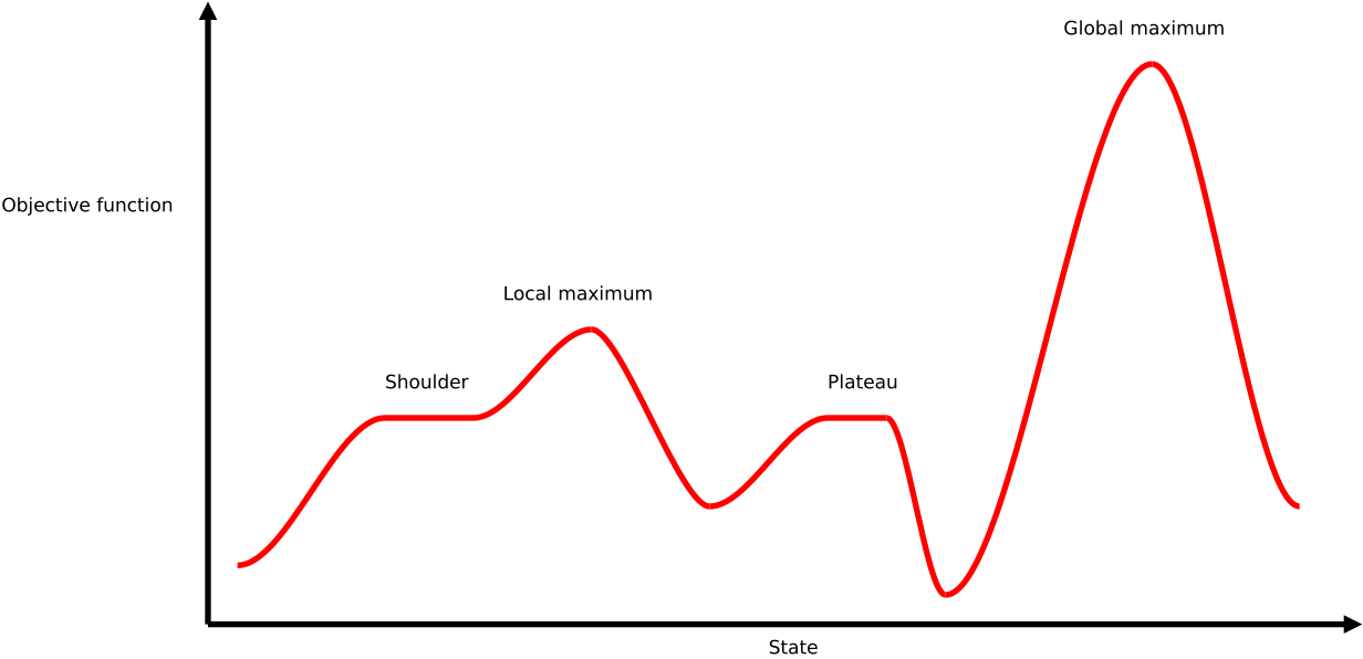
Problems with Hill Climbing:
Local Maxima: All neighbors worse, but not globally optimal
Plateaus: Flat regions where all neighbors have same value
Ridges: Sequence of local maxima difficult to navigate
Solutions:
Random restart: Try multiple random initial states
Stochastic hill climbing: Choose randomly among uphill moves
First-choice: Take first improvement found
Random walk: Sometimes take random steps
2.4.2 Simulated Annealing¶
Simulated annealing is a probabilistic optimization algorithm inspired by the annealing process in metallurgy. It allows occasional uphill moves (accepting worse solutions) to escape local optima.
Key Ideas:
Accept moves to worse solutions with a certain probability
This enables the search to escape local optima and explore more thoroughly
Since worse solutions can be accepted, the algorithm stores the best solution found during search
The probability of accepting worse solutions decreases over time (controlled by temperature)
Algorithm:
Algorithm: SimulatedAnnealing(Initial State s, Loss L, Schedule T(t))
begin
    current ← s
    best ← s
    T ← T₀  // Initial temperature (same magnitude as typical loss differences)
    t ← 1

    loop
        next ← random neighbor of current
        ΔL ← L(next) - L(current)

        if ΔL < 0 then
            current ← next  // Always accept improvement
        else
            // Accept with probability exp(-ΔL/T)
            with probability exp(-ΔL/T) do
                current ← next

        if L(current) < L(best) then
            best ← current

        t ← t + 1
        T ← T₀ / log(t + 1)  // Cool down

    until no improvement in best for N iterations
    return best
end
Acceptance Probability:
Temperature Schedule:
High T: Accept bad moves frequently (explore widely)
Low T: Accept bad moves rarely (exploit current region)
T → 0: Becomes hill climbing
Common Schedules:
Linear: T(t) = T₀ - αt
Exponential: T(t) = T₀ × γᵗ (γ < 1)
Logarithmic: T(t) = T₀ / log(t)
Worked example of the acceptance rule. Suppose the current tour has loss (length) 120 and a candidate neighbor has loss 125, so . At an early iteration with :
There is a 61% chance of accepting this slightly worse move — the search is still exploring broadly. Later, once the schedule has cooled to , the same move now has:
Almost never accepted. This is precisely how SA transitions smoothly from broad exploration (high , behaves like a random walk) to fine-grained hill climbing (low , behaves like greedy local search) — without ever changing the algorithm itself, only the temperature.
Properties:
✓ Can escape local optima
✓ Guaranteed to find global optimum (with slow enough cooling)
✓ Simple to implement
✗ Requires tuning temperature schedule
✗ May be slow to converge
2.4.3 Tabu Search¶
Tabu search is an advanced local search algorithm that enhances hill climbing by incorporating memory structures to avoid cycling back to previously visited solutions.
Key Idea: Maintain a list of “tabu” moves or solutions that are temporarily forbidden, allowing the search to explore new areas of the solution space and escape local optima.
Worked example. In 8-Queens, suppose moving the queen in column 3 from row 5 to row 2 reduces conflicts, so the search takes that move. Plain hill climbing could later find that moving it back from row 2 to row 5 “looks” like the best available neighbor again (e.g., after other queens moved) — creating an infinite 2-cycle. Tabu search instead records the reverse move (“column 3: row 2 → row 5”) on the tabu list for the next iterations, forbidding it. The search is forced to try a different queen/column instead, which is exactly what lets it escape the cycle that pure hill climbing would fall into.
Algorithm:
Algorithm: TabuSearch(Initial State s, Loss L, Tabu Size k)
begin
    current ← s
    best ← s
    tabu_list ← empty list  // The tabu list

    loop
        Add current to tabu_list

        // Find best unvisited neighbor
        if all neighbors of current are in tabu_list then
            break  // No valid moves

        next ← best neighbor not in tabu_list

        // May also accept tabu moves if they're better than best ever (aspiration)
        current ← next

        if L(current) < L(best) then
            best ← current

    return best
end
Enhanced Tabu Search Strategies:
Tabu List Size: Limit to fixed number of recent moves. If exceeded, remove oldest entry
Aspiration Criteria: Allow tabu moves if they result in solution better than any previously found
Intensification: Focus search on promising areas when good solutions are found
Diversification: Periodically jump to unexplored regions to explore new areas
Features:
Tabu List: Fixed-size memory of recent moves/states
Aspiration Criteria: Override tabu if solution is best so far
Diversification: Periodically jump to unexplored regions
Intensification: Focus search on promising regions
Advantages:
Escapes local optima by forbidding backtracking
Often finds better solutions than hill climbing
Balances exploration and exploitation
Disadvantages:
Requires tuning tabu list size
More complex than simpler methods
2.4.4 Other Metaheuristics (Brief Overview)¶
Hill Climbing, Simulated Annealing, Tabu Search, and Genetic Algorithms are the most commonly taught local search methods, but many other nature-inspired metaheuristics exist for optimization. Two of the most widely used:
Particle Swarm Optimization (PSO) — inspired by flocks of birds / schools of fish. A population (“swarm”) of candidate solutions (“particles”) moves through the search space; each particle’s velocity is updated based on (1) its own best-known position, (2) the swarm’s best-known position, and (3) inertia from its current velocity:
PSO works natively on real-valued search spaces (no encoding/decoding step needed) and is popular for continuous function optimization and neural network training.
Ant Colony Optimization (ACO) — inspired by ants finding shortest paths using pheromone trails. Artificial ants construct solutions step-by-step, probabilistically favoring edges with more pheromone; pheromone is reinforced on edges used by good solutions and evaporates over time. ACO is especially effective for graph/combinatorial problems like TSP and vehicle routing — the same problem class GAs with permutation encoding target, but ACO constructs solutions edge-by-edge rather than evolving a population via recombination.
Comparison: Local Search Methods¶
| Method | Escape Local Optima? | Memory | Best For |
|---|---|---|---|
| Hill Climbing | No | None | Simple problems, quick solutions |
| Random Restart | Yes | None | Many local optima |
| Simulated Annealing | Yes (probabilistic) | None | Large state spaces |
| Tabu Search | Yes (deterministic) | Tabu list | Avoiding cycles, structured problems |
| Genetic Algorithm | Yes | Population | Complex optimization |
| Particle Swarm Optimization | Yes | Velocity + personal/global best | Continuous optimization |
| Ant Colony Optimization | Yes | Pheromone trails | Graph/routing problems |
2.5 Genetic Algorithms¶
Genetic algorithms (GAs) borrow their paradigm from the process of biological evolution, working with a population of candidate solutions whose fitness is improved over generations through selection, recombination, and random variation.
Core Concepts¶
Chromosome (Individual): A candidate solution encoded in some representation (bits, real numbers, permutation, tree, ...)
Gene: A single component/position of a chromosome
Population: A set of chromosomes maintained and evolved together
Fitness Function: Measures how good a chromosome is at solving the problem
Generation: One full cycle of evaluate → select → crossover → mutate
Selection: Choose parents based on fitness (fitter individuals more likely to reproduce)
Crossover (Recombination): Combine two parents to create offspring by exchanging genetic material
Mutation: Random changes to a chromosome to maintain diversity and enable exploration
Before running a GA, we must decide how to encode a solution as a chromosome (§2.5.1), and then how to implement each operator (§2.5.2–2.5.4). The encoding constrains which crossover and mutation operators are valid — this is one of the most important design decisions in a GA.
2.5.1 Chromosome Encoding Schemes¶
Encoding is the process of representing a candidate solution as a chromosome the GA can manipulate. The encoding determines which crossover/mutation operators are valid, so it should be chosen first, based on the structure of the problem.
| Scheme | Gene Type | Example Chromosome | Typical Problems |
|---|---|---|---|
| Binary encoding | Bits (0/1) | 1 0 1 1 0 0 1 | Knapsack (item in/out), SAT, feature selection, classic function optimization |
| Real-value encoding | Floating-point numbers | [2.31, -0.87, 5.02] | Continuous parameter tuning, neural network weights, engineering design |
| Order (permutation) encoding | A permutation of symbols, no repeats | [3, 1, 4, 2, 5] | TSP, job-shop scheduling, timetabling — anything about ordering |
| Tree encoding | Tree of operators/operands | (x + 2) * y | Genetic Programming — evolving programs, mathematical expressions |
1. Binary encoding Each gene is a single bit. It is the original scheme used by Holland (1975) and remains popular for its simplicity, since bit-flip mutation and single-point crossover are trivial to implement.
Example — 0/1 Knapsack: chromosome
1011001means “include items 1, 3, 4, 7” (1 = in the sack, 0 = left out).Weakness: a numeric parameter (e.g. “weight in kg”) must first be discretized into bits, which introduces Hamming cliffs — e.g.
0111(7) and1000(8) differ in every bit even though the values are adjacent.
2. Real-value (continuous) encoding Each gene is a real number, used directly as a parameter — no binary decoding step needed.
Example — tuning 3 hyperparameters of a controller: chromosome
[2.31, -0.87, 5.02].Avoids Hamming cliffs and gives finer precision than a fixed-length bit string; requires different operators (arithmetic crossover, Gaussian mutation — see below).
3. Order / permutation encoding Each gene is a symbol (city, task, job) and the chromosome is a permutation — every symbol appears exactly once. Standard bit/real operators would produce invalid chromosomes (duplicated or missing symbols), so specialized operators are required (§2.5.3–2.5.4).
Example — TSP with 5 cities: chromosome
[3, 1, 4, 2, 5]means “visit city 3, then 1, then 4, then 2, then 5.”
4. Tree encoding Used in Genetic Programming (GP): the chromosome is an expression tree (operators as internal nodes, operands/constants as leaves) representing a program, formula, or decision rule.
Example: the tree for
(x + 2) * yevolves by swapping subtrees (crossover) or replacing a random subtree (mutation).Chromosomes can vary in size/shape, unlike the fixed-length schemes above.
2.5.2 Selection Operators¶
Selection decides which individuals in the current population become parents of the next generation. It drives the population towards fitter regions of the search space — the “survival of the fittest” step. All selection methods must balance two competing forces:
Selection pressure (favoring the best individuals) → faster convergence, but risks premature convergence to a local optimum
Diversity preservation (giving weaker individuals a chance) → slower convergence, but explores more of the search space
Roulette Wheel Selection (Fitness-Proportionate Selection)¶
Each individual is assigned a slice of a “roulette wheel” proportional to its fitness. The wheel is “spun” (a uniform random number is drawn) once per parent needed.
Worked example. Suppose a population of 4 chromosomes has these fitness values:
| Chromosome | Fitness | Probability | Cumulative | Expected count |
|---|---|---|---|---|
| A | 169 | 0.144 | 0.144 | 0.58 |
| B | 576 | 0.492 | 0.636 | 1.97 |
| C | 64 | 0.055 | 0.691 | 0.22 |
| D | 361 | 0.309 | 1.000 | 1.23 |
| Sum | 1170 | 1.00 | — | 4 |
To select one parent: draw and pick the first chromosome whose cumulative probability is . E.g. falls between C’s (0.691) and D’s (1.000) cumulative bounds → D is selected. Repeating this times fills the mating pool; chromosome B (highest fitness) is expected to be picked about twice as often as D, and roughly 9× more often than C.
Weakness: if one chromosome dominates fitness (e.g. vs. others ), it takes over the wheel and the population converges prematurely. If all fitness values are close together, selection pressure is too weak and the search behaves almost like random selection — this is exactly the problem rank-based selection fixes below.
Rank-Based Selection¶
Instead of using raw fitness, individuals are first sorted by fitness and assigned a selection probability based on their rank, not their fitness magnitude. This fixes roulette wheel’s two failure modes (domination by super-individuals, or too-flat a distribution).
For linear ranking with selective pressure , rank (worst) … (best):
Example with our 4 chromosomes ranked worst→best as C, A, D, B and (maximum pressure): probabilities become approximately — a smooth, controlled gradient regardless of how extreme the raw fitness gap was.
✓ Robust to outliers and fitness scaling
✗ Loses information about how much fitter one individual is; requires an sort every generation
Tournament Selection¶
Pick individuals uniformly at random from the population (tournament size) and select the fittest one among them. Repeat to refill the mating pool.
Example (): randomly draw {A, C, D} → fitnesses {169, 64, 361} → winner = D.
Larger → higher selection pressure (best individuals win almost every tournament) → faster but riskier convergence
Smaller (e.g. ) → more diversity retained, gentler pressure
✓ No global fitness scaling needed, trivially parallelizable, pressure is tunable via — this is why it’s the most widely used selection method in practice (it’s what the N-Queens GA implementation in this book uses)
Steady-State Selection¶
Rather than replacing the entire population every generation (a generational GA), steady-state selection replaces only a small number of individuals (often just 1–2) per iteration: select 2 parents → produce 1–2 offspring → replace the worst individual(s) currently in the population.
✓ Naturally preserves elite solutions (implicit elitism), can converge faster on some problems
✗ Higher risk of premature convergence and loss of diversity; must actively manage duplicates
Comparison of Selection Operators¶
| Method | Selection Pressure | Diversity | Cost | Best For |
|---|---|---|---|---|
| Roulette Wheel | Depends on fitness spread (can be too high or too low) | Medium | Simple, well-scaled fitness landscapes | |
| Rank-Based | Controlled/tunable () | High | Fitness values vary wildly, or population has converged (flat fitness) | |
| Tournament | Tunable via | High (small ) | General purpose — most popular in modern GAs | |
| Steady-State | High | Low (needs management) | per replacement | Continuous/online evolution, real-time or streaming problems |
2.5.3 Crossover Operators¶
Crossover (recombination) combines the genetic material of two parents to produce offspring that (hopefully) inherit the best traits of both. It is the primary exploitation operator — it recombines existing building blocks rather than inventing new genetic material (that’s mutation’s job). The valid crossover operators depend entirely on the encoding chosen in §2.5.1.
Crossover for Binary / Real-Value Encoding¶
1. Single-point crossover — pick one random cut point; swap the tails after it.
Parent 1:  1 0 1 | 1 0 0 1        Child 1:  1 0 1 | 0 1 1 0
Parent 2:  0 1 0 | 0 1 1 0        Child 2:  0 1 0 | 1 0 0 1
                ^ cut point
2. Two-point crossover — two cut points; swap only the middle segment. Reduces “positional bias” (single-point crossover always disrupts genes near the ends less than genes in the middle).
Parent 1:  1 0 | 1 1 0 | 0 1      Child 1:  1 0 | 0 1 1 | 0 1
Parent 2:  0 1 | 0 0 1 | 1 0      Child 2:  0 1 | 1 1 0 | 1 0
3. Uniform crossover — for each gene independently, flip a coin to decide which parent it comes from (mask-driven). Much more disruptive/exploratory than 1- or 2-point crossover, since it can mix genes at every position.
Mask:      1 0 1 0 0 1 1          (1 = take from Parent 1, 0 = take from Parent 2)
Parent 1:  1 0 1 1 0 0 1
Parent 2:  0 1 0 0 1 1 0
Child:     1 1 1 0 1 0 1
4. Arithmetic crossover (real-valued only) — child genes are a weighted average of the parents:
E.g. parent₁ = [2.0, 4.0], parent₂ = [6.0, 0.0], → child = [5.0, 1.0]. Unlike the other operators, this can create values between the parents’ genes rather than just recombining existing bits.
Crossover for Permutation Encoding¶
Order Crossover (OX1) — copies a random slice from Parent 1 directly, then fills the remaining positions with the missing cities from Parent 2, in the order they appear, skipping duplicates.
Parent 1:  1 2 | 3 4 5 6 | 7 8
Parent 2:  3 7 | 5 1 6 8 | 2 4
                 ^ copy this slice from P1 into the child: _ _ 3 4 5 6 _ _

Remaining cities needed (in Parent 2's order, skipping 3,4,5,6): 7 1 8 2
Fill child's empty slots left-to-right with this sequence:

Child:     7 1 | 3 4 5 6 | 8 2
Partially Mapped Crossover (PMX) — like OX1, copies a slice from Parent 1, but resolves the remaining positions using a mapping between the swapped segments of both parents (position in Parent 2’s slice maps to the value at position in Parent 1’s slice), guaranteeing a valid permutation while preserving more absolute position information than OX1.
Cycle Crossover (CX) — identifies cycles of corresponding positions/values between the two parents (following “value at position in P2 → find that value’s position in P1 → ...”) and each cycle is copied entirely from one parent, alternating parents cycle-by-cycle. This preserves the absolute position of as many genes as possible.
| Operator | Preserves | Best For |
|---|---|---|
| OX1 | Relative order of cities | TSP, general sequencing |
| PMX | Absolute positions where possible | Problems where position matters (e.g. timetable slots) |
| CX | Absolute position, using every gene from one parent or the other | Problems needing strict position inheritance |
2.5.4 Mutation Operators¶
Mutation randomly perturbs a chromosome to introduce genetic material that did not exist in the population before — this is the GA’s main exploration operator, applied with low probability so it doesn’t destroy good solutions found by crossover. Like crossover, the valid mutation operators depend on the encoding.
| Encoding | Operator | Mechanism | Example |
|---|---|---|---|
| Binary | Bit-flip | Each bit flips (0↔1) independently with probability | 1011001 → 1010001 |
| Real-valued | Uniform mutation | Replace a gene with a new random value in its allowed range | [2.31, -0.87] → [2.31, 3.14] |
| Real-valued | Gaussian (creep) mutation | Add small noise to a gene — fine-tunes near an optimum | 5.02 → 5.02 + 0.03 = 5.05 |
| Permutation | Swap mutation | Pick two positions, swap their values | [3,1,4,2,5] → [3,1,5,2,4] |
| Permutation | Insertion mutation | Remove a gene, reinsert at a random position | [3,1,4,2,5] → [3,4,2,1,5] |
| Permutation | Scramble mutation | Pick a subsequence, shuffle it randomly | [3,1,4,2,5] → [3,2,1,4,5] |
| Permutation | Inversion mutation | Pick a subsequence, reverse its order | [3,1,4,2,5] → [3,4,1,2,5] |
| Tree (GP) | Subtree mutation | Replace a randomly chosen subtree with a new random subtree | (x+2)*y → (x+2)*(y-1) |
Why inversion mutation matters for TSP: reversing a segment of a tour is exactly the classic 2-opt local-search move — it only changes 2 edges of the tour, making it a much gentler perturbation than swap mutation (which can change up to 4 edges). This is why inversion is often preferred over swap for routing problems.
Mutation rate : typically small (0.001–0.05 per gene for bit-flip, or a fixed per-chromosome probability like 0.1–0.2 for swap/inversion, as used in the N-Queens implementation). Too high and the GA degenerates into random search; too low and the population can get stuck (premature convergence, especially combined with high-pressure selection).
2.5.5 Crossover vs. Mutation: Exploitation vs. Exploration¶
Although both are “genetic operators,” crossover and mutation play very different roles in balancing the GA’s search:
| Aspect | Crossover | Mutation |
|---|---|---|
| Role | Exploitation — recombines existing good building blocks | Exploration — introduces novel material not in the population |
| Parents needed | 2 (or more) | 1 |
| Applied with probability | High, –0.9 | Low, –0.05 (per gene) |
| Typical effect size | Large jump (recombines whole segments) | Small, local perturbation |
| If rate too high | Population loses diversity fast around a few strong schemas → premature convergence | Search degenerates into pure random search |
| If rate too low | Little recombination → slow progress, relies solely on mutation | Population stagnates once diversity is lost → stuck in local optimum |
2.5.6 Putting It All Together: One Generation by Hand¶
Consider the classic problem of maximizing for integer , using 5-bit binary encoding (so ranges over all values representable in 5 bits).
Step 1 — Initial population (encoding):
| Chromosome | (decoded) | Fitness |
|---|---|---|
01101 | 13 | 169 |
11000 | 24 | 576 |
01000 | 8 | 64 |
10011 | 19 | 361 |
Step 2 — Selection (roulette wheel, from §2.5.2): using the probabilities computed earlier (A=0.144, B=0.492, C=0.055, D=0.309), four spins might select the mating pool {B, B, D, A} — chromosome C (weakest) was not selected at all, while B (fittest) was selected twice.
Step 3 — Crossover (single-point, ): pair up (B, B) and (D, A); suppose (D, A) crosses after bit 3:
D: 100|11        Child: 100|01  (= 9,  f = 81 — worse, but adds diversity)
A: 011|01        Child: 011|11  (= 15, f = 225)
(B, B) are identical, so crossover produces no change — this pair passes through unmodified.
Step 4 — Mutation (bit-flip, per bit): suppose bit 4 of 11000 flips: 11000 → 11010 (26, — an improvement!).
Step 5 — New population & fitness: {11000, 11010, 10001, 01111} → fitnesses {576, 676, 81, 225}. The best fitness improved from 576 → 676 in a single generation, driven by a lucky mutation — this illustrates exactly why mutation matters even though crossover does most of the work on average.
General Algorithm:
Algorithm: GeneticAlgorithm(Population Size N, Generations T)
begin
    population ← random initialization of N chromosomes (using chosen encoding)
    t ← 1

    repeat
        Evaluate fitness of each chromosome

        // Select parents based on fitness (roulette / rank / tournament / steady-state)
        mating_pool ← Select(population)

        // Crossover to create offspring (operator depends on encoding)
        offspring ← Crossover(mating_pool, p_c)

        // Mutate with some probability (operator depends on encoding)
        offspring ← Mutate(offspring, p_m)

        population ← offspring  // (or replace worst, for steady-state)
        t ← t + 1
    until convergence condition is met

    return best chromosome from population
end
Example: TSP with GAs
Encoding: Permutation of cities
[3,1,4,2,5]representing tour orderFitness: Negative of tour length (shorter tours = higher fitness)
Selection: Tournament selection is most common
Crossover: Order crossover (OX1) — preserves relative city order from parents
Mutation: Inversion or swap mutation — reversing/swapping a segment of the tour