Introduction to Multiagent Environments
Multiagent environments contain several decision-makers whose actions influence one another. In single-agent search, the agent only needs to reason about the environment. In multiagent search, the environment includes other agents that may cooperate, compete, or act independently.
This changes the nature of planning: the agent is no longer looking for a fixed sequence of actions, but for a strategy that remains sensible under different responses from others.
Key Challenges:
Other agents may have different goals, information, and capabilities.
The effect of one action depends on how other agents respond.
Planning often requires contingency reasoning rather than a single straight-line plan.
Search can grow much faster because each turn introduces multiple possible reactions.
Why Multiagent Search Is Different
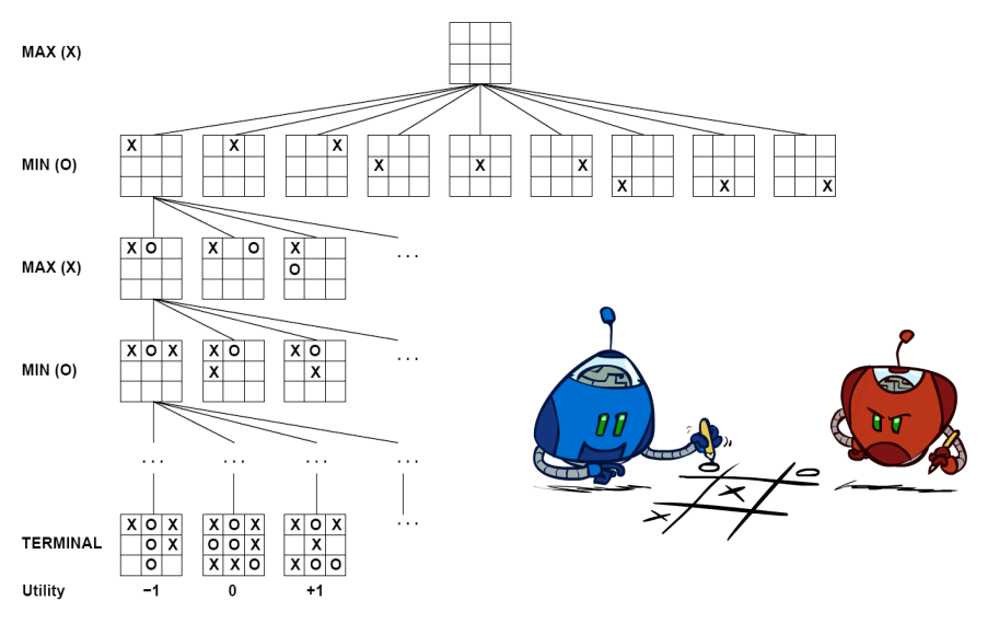
Consider Tic-Tac-Toe. In a single-agent puzzle, once you choose an action, the next state is determined by the environment rules. In Tic-Tac-Toe, after you place an X, the opponent chooses where to place O. Your move does not define one future, it defines a set of possible futures.
That is why multiagent search needs special tree structures:
At your turn, you choose among alternatives.
At an opponent’s turn, you must account for their possible responses.
In adversarial settings, a good move is one that still leads to a strong outcome even when the opponent plays well.
This is the central shift from plan finding to strategy selection.
Types of Multiagent Environments
Competitive agents Agents pursue conflicting objectives. One agent’s gain may reduce the other’s payoff. This is the setting for adversarial search. Examples: Chess, Go, Tic-Tac-Toe
Independent agents Agents act without explicit coordination. Their decisions still affect one another, even if they do not communicate. Example: Self-driving cars navigating traffic
Cooperative agents Agents share information or align their objectives to improve a joint outcome. Example: Collaborative robots in a warehouse, team-based rescue systems
A chapter on multiagent search should keep these distinctions in mind because the right search method depends on the relationship between agents.
Uninformed Search: AND-OR Search Trees
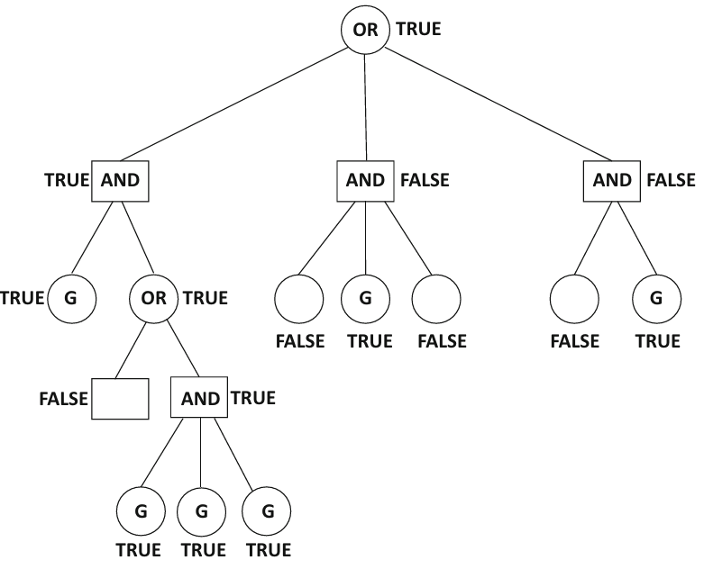
AND-OR search trees model situations where outcomes depend both on our decisions and on the responses of other agents or the environment.
OR nodes represent states where our agent chooses one action from several alternatives.
AND nodes represent states where the next outcome depends on responses outside our control, so the plan must work for every relevant continuation.
In adversarial settings, OR nodes correspond to our move and AND nodes correspond to the opponent’s possible replies. In nondeterministic planning, AND nodes can also represent uncertain environmental outcomes.
The key idea is simple: at an OR node we need one good choice, while at an AND node we must be ready for all relevant outcomes.
AO-Search Algorithm
The AO-Search algorithm traverses an AND-OR tree to find a guaranteed path to a goal state.
def ao_search(state, goal_test):
    # If current state is a goal, return True
    if goal_test(state):
        return True
    # If state is an OR node (our turn)
    if state.is_or_node():
        # We need to find just ONE successful action
        for action in state.get_actions():
            next_state = state.get_next(action)
            if ao_search(next_state, goal_test):
                return True # Found a winning path
        return False # No winning action from this state
    # If state is an AND node (opponent's turn)
    else:
        # We need to handle ALL opponent responses
        for action in state.get_actions():
            next_state = state.get_next(action)
            if not ao_search(next_state, goal_test):
                return False # Opponent has a move that makes us lose
        return True # We can win regardless of opponent's move
The AND-OR Tree for Multiagent Search
The figure below illustrates the main structural idea: our agent chooses at OR nodes, while the plan must remain valid across the outcomes represented at AND nodes.
Handling More than Two Agents
What happens in settings where there are more than two agents?
The AND-OR tree structure can be extended to accommodate multiple agents by alternating between AND and OR nodes for each agent’s turn. Each AND node would represent the choices of all other agents, while each OR node would represent the choices of the current agent. For example, in a three-agent game (A, B, C):
OR nodes: Represent the choices of agent A.
AND nodes: Represent the combined choices of agents B and C.
This structure allows us to systematically explore the possible outcomes based on the actions of all agents involved.
Combining multiple actions into a single action can blow up the number of possible actions at a particular state.
This will result in a tree with very high degree, whose size increases rapidly with increasing depth.
Informed Search Trees with State-Specific Evaluation Functions
In large games such as chess, Go, or strategic board games, exploring the full search tree is usually impossible. The branching factor is too high and the game may last too long.
To make search practical, agents estimate the quality of non-terminal states using an evaluation function. Instead of asking, “Who wins from here if we search to the end?” the agent asks, “How promising does this state look right now?”
This idea enables depth-limited search: search several moves ahead, stop before the tree becomes too large, and score the frontier states using the evaluation function.
Core Terminology and Notation
Before moving to informed search, it is useful to fix the vocabulary used throughout the chapter:
State: a configuration of the game or environment.
Action: a legal move available to the current agent.
Terminal state: a state where the interaction ends and a final payoff is known.
Utility: a score where larger values are better for the maximizing agent.
Loss or cost: a score where smaller values are better for the acting agent.
Evaluation function: an estimate of how good a non-terminal state is when we cannot search to the end.
MAX / MIN: the two roles used in adversarial search, where MAX tries to increase value and MIN tries to reduce it.
Using these terms consistently prevents confusion when the chapter moves from AND-OR search to minimax and Monte Carlo Tree Search.
Designing State-Specific Evaluation Functions
Evaluation functions are built from features that matter in a domain. In chess, for example, a heuristic may combine material advantage, king safety, center control, and piece activity.
These functions are powerful but imperfect:
They summarize a rich position using a limited set of features.
They may miss tactical ideas that only appear deeper in the tree.
Their quality strongly influences the quality of the decisions produced by search.
In adversarial games, evaluation is often aligned with utility. If one player’s gain is the other’s loss, a single scoring function can often be interpreted from opposite perspectives. In more general multiagent settings, each agent may have its own objective, so the relationship between scores may be weaker or unknown.
Depth-Limited Search
Depth-limited search cuts off expansion after a chosen depth and then applies an evaluation function at the frontier.
This is a practical compromise:
Searching deeper usually improves decision quality.
Searching too deeply can be computationally infeasible.
Better evaluation functions can partly compensate for shallower search.
In practice, strong game-playing systems combine both ingredients: enough lookahead to capture tactical consequences, and enough evaluation quality to rank non-terminal positions sensibly.
Two-Agent Search with Evaluation Functions
The following simplified pseudocode uses loss values, where smaller numbers are better for the current agent. This avoids confusion: both agents choose the continuation that minimizes their own future loss.
def search_agent_a(state, depth):
    if depth == 0 or is_terminal(state):
        return loss_for_a(state)

    best_loss = float("inf")
    for next_state in successors(state):
        reply_loss = search_agent_b(next_state, depth - 1)
        best_loss = min(best_loss, reply_loss)
    return best_loss

def search_agent_b(state, depth):
    if depth == 0 or is_terminal(state):
        return loss_for_b(state)

    best_loss = float("inf")
    for next_state in successors(state):
        reply_loss = search_agent_a(next_state, depth - 1)
        best_loss = min(best_loss, reply_loss)
    return best_loss
The important point is that each agent evaluates future states through its own objective function. In zero-sum games, this eventually leads to the cleaner MAX/MIN formulation used by minimax.
Informed Search: Minimax for Adversarial Search
Minimax is the standard algorithm for two-player, zero-sum, deterministic games with perfect information. It assumes both players act rationally and play optimally.
MAX tries to maximize the utility value.
MIN tries to minimize the utility value.
Terminal states provide the true payoff.
Non-terminal states inherit their value from the best move of the player whose turn it is.
This makes minimax a model of perfect play: it does not search for a lucky line, it searches for the best outcome that can still be guaranteed against a strong opponent.
Minimax: MaxPlayer and MinPlayer Algorithms
The algorithm is naturally expressed through two mutually recursive procedures.
MaxPlayer Algorithm
def max_player(state, depth):
    if depth == 0 or is_terminal(state):
        return utility(state)

    best_value = -infinity
    for action in get_actions(state):
        next_state = get_next_state(state, action)
        child_value = min_player(next_state, depth - 1)
        best_value = max(best_value, child_value)
    return best_value
MinPlayer Algorithm
def min_player(state, depth):
    if depth == 0 or is_terminal(state):
        return utility(state)

    best_value = +infinity
    for action in get_actions(state):
        next_state = get_next_state(state, action)
        child_value = max_player(next_state, depth - 1)
        best_value = min(best_value, child_value)
    return best_value
The alternation matters: MAX assumes MIN will answer with the move that is worst for MAX, and MIN assumes MAX will answer with the move that is best for MAX.
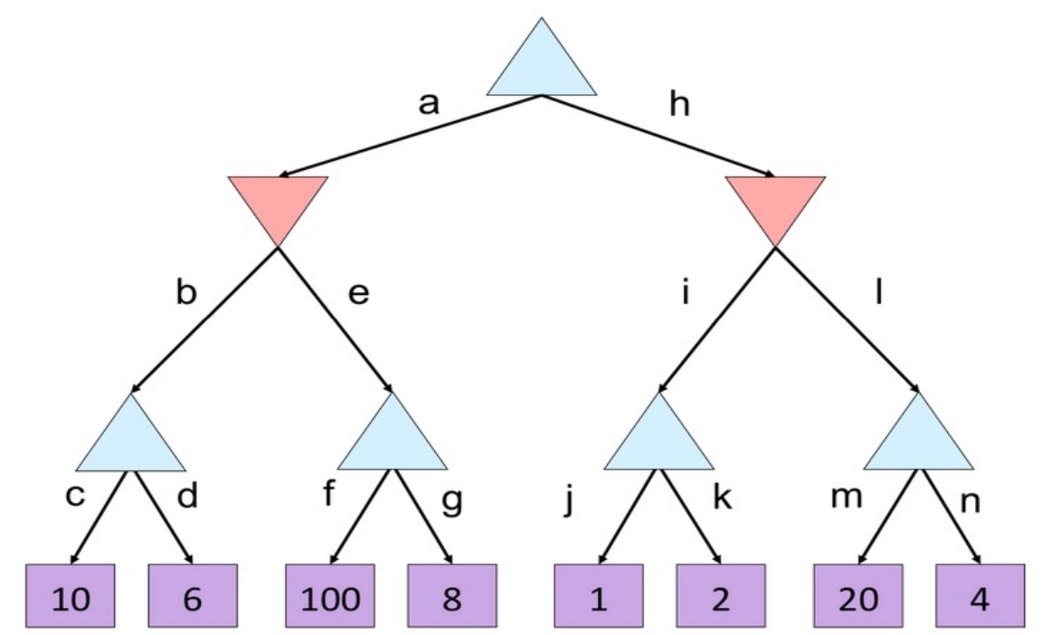
Minimax Example
Read the tree from the leaves upward:
The left MIN node chooses .
The middle MIN node chooses .
The right MIN node chooses .
The root MAX node then chooses .
So MAX selects the left branch, not because it has the largest leaf anywhere in the tree, but because it has the best value after accounting for MIN’s best possible reply.
Alpha-Beta Pruning
Alpha-beta pruning improves minimax by avoiding branches that cannot affect the final choice. It returns the same answer as minimax, but often explores far fewer nodes.
is the best value MAX can guarantee so far.
is the best value MIN can guarantee so far.
If at any point , the remaining descendants of that branch cannot change the decision and may be pruned.
A critical practical point is move ordering: alpha-beta is most effective when strong moves are examined early, because early good bounds create more opportunities to prune later branches.
Alpha-Beta Pruning Quiz
Use the figure below to identify where pruning should occur and which nodes never need evaluation if the tree is explored from left to right.
A good way to solve this kind of problem is to track and after every visited child rather than trying to guess the answer visually.
Alpha-Beta Pruning Quiz Solution
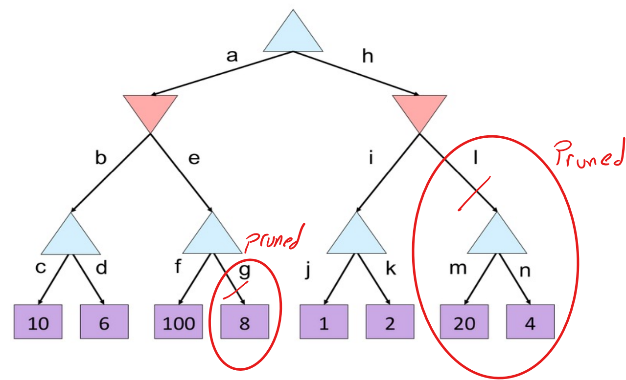
The main lesson is not just where pruning occurs, but why it occurs: once a node is already worse than an alternative found earlier, further exploration cannot improve the final decision at the parent.
Monte Carlo Tree Search (MCTS)
Monte Carlo Tree Search is an inductive search method that estimates which moves are promising by repeated simulation rather than exhaustive evaluation. It is especially useful when the branching factor is very large or when a handcrafted evaluation function is difficult to design.
Why MCTS works well in practice:
It focuses computation on promising parts of the tree.
It is an anytime algorithm: more simulations usually improve the estimate.
It does not require searching every branch to the same depth.
The four phases of MCTS are:
Selection: Traverse the current tree using a rule such as UCT.
Expansion: Add a new child after reaching a frontier node.
Simulation: Run a rollout from that node to estimate outcome quality.
Backpropagation: Update visit counts and rewards along the path back to the root.
UCT Formula: The Upper Confidence Bound for Trees balances exploitation and exploration:
: number of wins or accumulated reward for node
: number of visits to node
: number of visits to the parent of node
: exploration parameter
Compared with minimax, MCTS is often a better fit when evaluation is uncertain but simulations are cheap enough to provide useful statistical guidance.
Choosing the Right Search Method
| Situation | Recommended Method | Reason |
|---|---|---|
| Contingent planning with uncertain outcomes | AND-OR search / AO-search | The solution must account for multiple possible continuations. |
| Two-player adversarial game with manageable depth | Minimax | Gives the optimal decision under perfect play assumptions. |
| Same adversarial setting but deeper trees | Alpha-beta pruning | Preserves minimax correctness while reducing search effort. |
| Very large branching factor or weak heuristic design | MCTS | Uses simulation to focus computation on promising moves. |
This comparison matters in practice because no single search method dominates across all multiagent settings. The right algorithm depends on whether the environment is adversarial, uncertain, cooperative, or simply too large for exhaustive search.
Applications Beyond Board Games
Multiagent search is not limited to games. The same ideas appear in several AI application domains:
Autonomous driving: a vehicle must choose actions while anticipating how nearby drivers may react.
Cybersecurity: a defender plans under the assumption that an attacker will actively search for weaknesses.
Robotics: teams of robots may coordinate to complete a shared task, or adversarial robots may block one another.
Economics and auctions: agents place bids or adjust prices while reasoning about strategic competitors.
These applications remind us that multiagent search is fundamentally about decision-making in the presence of other intelligent actors.
Practice Prompts
Draw a small AND-OR tree for a robot trying to reach a goal while an opponent blocks paths.
Evaluate a depth-2 minimax tree by propagating leaf values from the bottom up.
Show where alpha-beta pruning occurs when children are explored from left to right.
Explain why MCTS may outperform minimax in games with huge branching factors.
These short exercises are useful because they force you to apply each idea rather than only recognize the terminology.
Summary
Multiagent search differs from single-agent search because good decisions must account for the responses of other agents.
AND-OR trees model contingent reasoning, where some branches represent our choices and others represent outcomes we must be prepared for.
Evaluation functions make large search problems tractable by estimating the quality of non-terminal states.
Minimax gives the correct move under perfect-play assumptions in two-player zero-sum games.
Alpha-beta pruning preserves the minimax answer while cutting unnecessary search.
MCTS is often preferable when the tree is too large for exhaustive reasoning and simulation is informative.
Real-world AI systems often combine search, heuristics, and learning rather than relying on only one technique.