2.1 Introduction
Search is one of the most fundamental problem-solving techniques in artificial intelligence. Many AI problems can be formulated as finding a sequence of actions that transforms an initial state into a goal state.
Core Concept
The goal of an agent is to:
Start from an initial state
Perform a sequence of actions
Reach a goal state (or a state with high desirability)
Two Main Scenarios
Goal-Oriented Search: Find a path from start to goal
Example: Solving a maze, solving a puzzle
Cost may be associated with paths
Optimization Search: Find state with minimal loss
Example: Eight-queens placement, scheduling
Cost is associated with states themselves
Applications
Why Search Matters
No Direct Formula: Many problems have no closed-form solution
Large Solution Space: Too many possibilities to enumerate
Need Systematic Methods: Avoid aimless wandering
Trade-offs: Different strategies balance time, memory, and solution quality
2.1.1 State Space as a Graph
Modeling the state space as a directed graph enables systematic search:
Key Concepts:
Node: Represents a state
Edge: Represents a transition (action) from one state to another
Path: Sequence of edges from initial state to goal
Example: Eight-Queens Problem
Problem: Place 8 queens on a chessboard so none attack each other.
State Space Design:
Approach 1 (Incremental):
State: Placement of k ≤ 8 queens (no attacks)
Action: Add one more queen
Initial State: Empty board (k=0)
Goal State: 8 queens placed (k=8)
Graph Type: Directed Acyclic Graph (DAG)
Approach 2 (Complete State):
State: Any placement of 8 queens (attacks allowed)
Action: Move one queen to different square
Initial State: Random placement
Goal State: No attacks
Graph Type: Undirected graph with cycles
State Space Size
| Problem | State Space Size |
|---|---|
| 8-Queens (any placement) | 64C8 ≈ 4.4 × 10⁸ |
| 8-Puzzle | 9! = 362,880 |
| Chess (valid positions) | > 10⁴³ |
| Rubik’s Cube | ≈ 4.3 × 10¹⁹ |
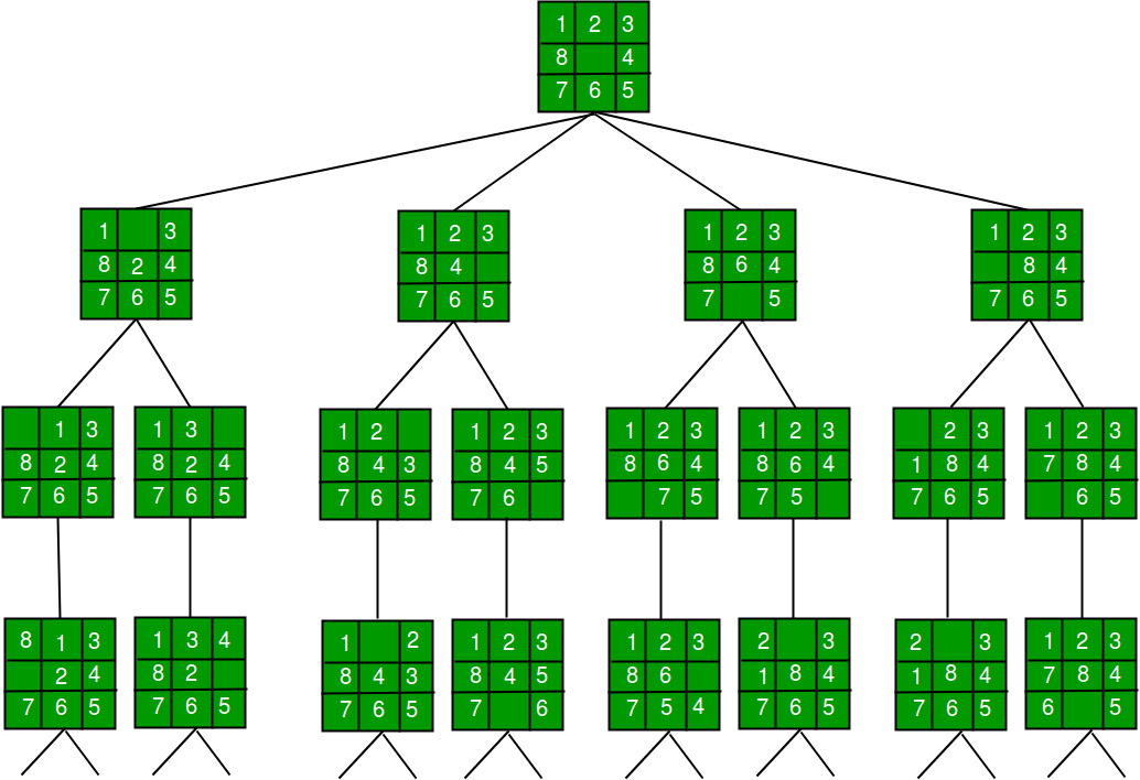
2.1.2 Search Space vs Search Tree
The state space graph represents all possible states and transitions in the problem domain, while the search tree represents the specific paths taken during the search process.
Key Differences:
| Aspect | State Space Graph | Search Tree |
|---|---|---|
| Definition | All possible states and transitions | Paths explored by search algorithm |
| Duplicates | Each state appears once | Same state may appear multiple times |
| Size | Fixed by problem | Can be infinitely larger |
| Cycles | May contain cycles | Represents unrolled paths |
Example: State Space Graph
Corresponding Search Tree:
The search tree unfolds paths from the root, potentially duplicating states reached via different paths.
Example with Cycles:
Consider a graph:
State Space: 4 nodes (S, a, b, G)
Search Tree: Could expand infinitely
This is why search algorithms must track visited states to avoid infinite loops!
2.1.3 Search Problem Examples
Example 1: Pacman
Problem: Navigate Pacman through a maze to collect all food pellets.
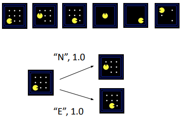
State Space Design:
State: Pacman’s current position + remaining food pellets
Successor Function: Moving in one of four cardinal directions (N, E, S, W)
Start State: Pacman at initial position with all food pellets present
Goal Test: All food pellets have been collected
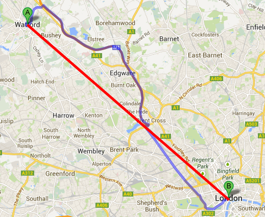
Example 2: Traveling in Romania
Problem: Find the shortest route between cities.
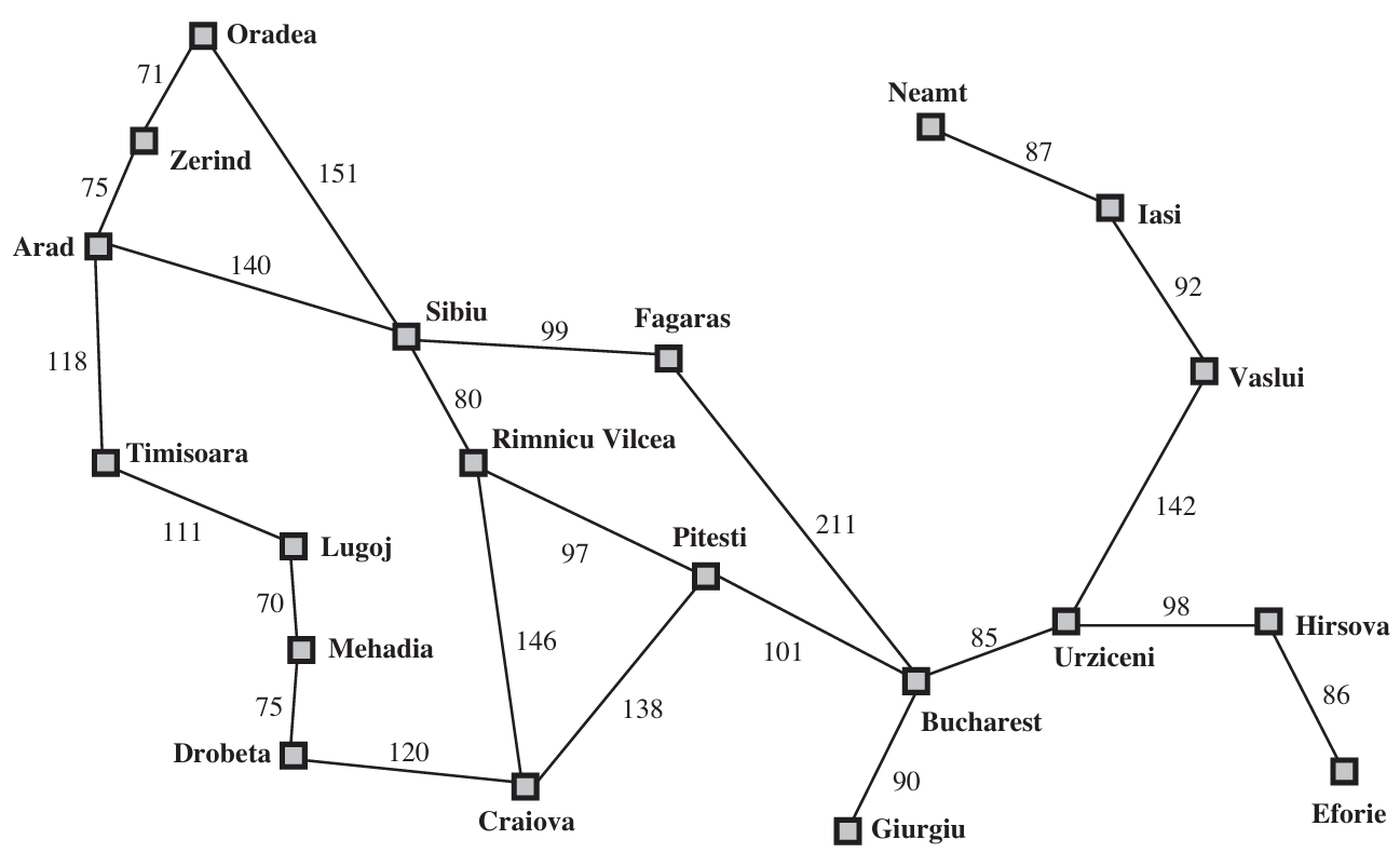
State Space Design:
State: Current city location
Successor Function: Moving from one city to another connected by a road (cost = distance)
Start State: Initial city (e.g., Arad)
Goal Test: Reaching destination city (e.g., Bucharest)
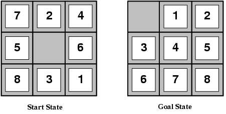
Example 3: Eight-Puzzle
Problem: The Eight-Puzzle is a sliding puzzle that consists of a 3x3 grid with eight numbered tiles and one empty space. The objective is to arrange the tiles in a specific order by sliding them into the empty space.
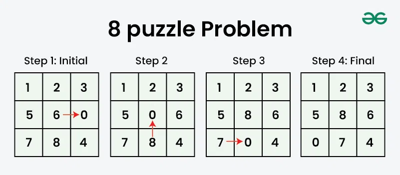
State Space Design:
State: Configuration of tiles on the 3×3 board
Successor Function: Sliding a tile into the empty space
Start State: Initial scrambled configuration
Goal Test: Tiles arranged in desired order (1-8 with blank in corner)
Example 4: Online Maze Search
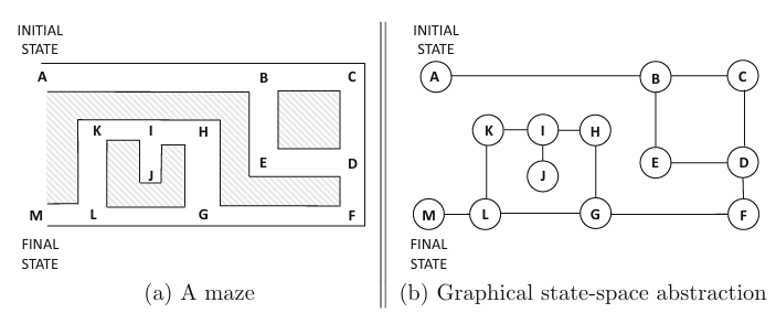
State Space Design:
State: Agent’s current position in the maze
Successor Function: Moving in one of four cardinal directions (up, down, left, right) based on current position and maze layout
Start State: Initial position in the maze
Goal Test: Reaching the exit of the maze
2.2 Uninformed Search Algorithms
Uninformed search algorithms, also known as blind search algorithms, are a category of search strategies that operate without any domain-specific knowledge about the problem being solved. They explore the search space systematically, relying solely on the structure of the state space and the goal test to find a solution.
Generic Search Framework
All uninformed search algorithms follow this template:
Algorithm: GenericSearch(Initial State s, Goal Condition G)
Input: Initial state s, Goal condition G
Output: Path from s to goal, or failure

begin
    LIST ← {s}              // Frontier nodes to explore
    VISIT ← ∅               // Visited nodes
    pred ← empty array      // Predecessor tracking

    repeat
        if LIST is empty then
            return failure

        // Selection strategy differs by algorithm
        Select node i from LIST
        Delete i from LIST
        Add i to VISIT

        if i satisfies G then
            return reconstruct_path(pred, s, i)

        // Expand node i
        for each node j adjacent to i do
            if j not in VISIT and j not in LIST then
                Add j to LIST
                pred[j] ← i
    until LIST is empty or goal found
end
Key Components:
LIST: Frontier nodes (boundary of explored region)
VISIT: Already explored nodes
pred: Predecessor array to reconstruct path
Selection Strategy: Determines which algorithm we get
2.2.1 Breadth-First Search (BFS)
BFS explores nodes level by level, visiting all nodes at depth d before any node at depth d+1.
Selection Strategy: FIFO queue (First-In-First-Out)
How it works:
Start with initial state in queue
Remove first node from queue
Check if it’s a goal
Add all unvisited neighbors to end of queue
Repeat
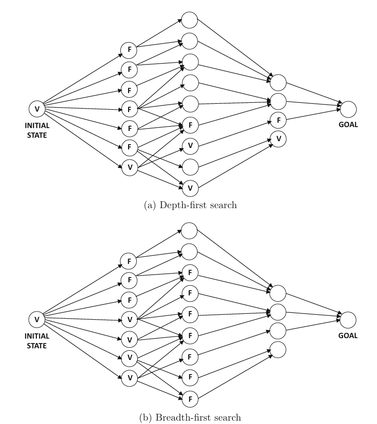
BFS Exploration Pattern:
Properties:
| Property | Value | Explanation |
|---|---|---|
| Complete | Yes | Will find solution if one exists |
| Optimal | Yes* | Finds shallowest (shortest path) goal |
| Time Complexity | O(b^d) | Exponential in depth |
| Space Complexity | O(b^d) | Must store entire frontier |
*Only when all actions have equal cost
Where:
b: branching factor (average number of successors)
d: depth of shallowest goal
Advantages:
Guaranteed to find solution
Finds shortest path (minimum edges)
Disadvantages:
Memory intensive: Must store all nodes at current level
Slow for deep goals
2.2.2 Depth-First Search (DFS)
DFS explores as deep as possible along each branch before backtracking.
Selection Strategy: LIFO stack (Last-In-First-Out)
How it works:
Start with initial state on stack
Pop top node from stack
Check if it’s a goal
Push all unvisited neighbors onto stack
Repeat
DFS Exploration Pattern:
Properties:
| Property | Value | Explanation |
|---|---|---|
| Complete | No | Can get stuck in infinite paths |
| Optimal | No | May find longer paths first |
| Time Complexity | O(b^m) | Can explore entire tree |
| Space Complexity | O(bm) | Only stores single path |
Where:
m: maximum depth of any node
Advantages:
Memory efficient: Only stores nodes on current path
Fast if solutions are deep
Disadvantages:
Can get stuck in infinite loops (needs cycle detection)
May find suboptimal solutions
Not complete in infinite spaces
Comparison: BFS vs DFS
| Aspect | BFS | DFS |
|---|---|---|
| Frontier Shape | Wide, shallow | Deep, narrow |
| Memory | O(b^d) - HIGH | O(bm) - LOW |
| Optimal | Yes (equal costs) | No |
| Complete | Yes | No (with cycles) |
| Best For | Shallow goals | Deep solutions, memory limited |
2.2.3 Uniform-Cost Search (UCS)
UCS generalizes BFS to handle weighted graphs where actions have different costs. It is an uninformed search algorithm that expands the least costly node first, ensuring that the path to the goal is optimal in terms of cost. It uses a priority queue to manage the frontier, where nodes are prioritized based on their cumulative cost from the start state.
Selection Strategy: Priority queue ordered by path cost g(n)
Key Idea: Always expand the node with the lowest cumulative path cost from start.
Path Cost: g(n) = sum of edge costs from start to node n
How it works:
Maintain priority queue of nodes, ordered by g(n)
Always expand node with smallest g(n)
Update costs when shorter paths are found
Detailed Example:
After UCS execution:
Properties:
| Property | Value |
|---|---|
| Complete | Yes |
| Optimal | Yes |
| Time Complexity | O(b^(C*/ε)) |
| Space Complexity | O(b^(C*/ε)) |
Where:
C*: cost of optimal solution
ε: minimum edge cost
2.2.5 Bidirectional Search
Run two simultaneous searches: one forward from start, one backward from goal. Stop when they meet.
Key Idea: Two small searches are faster than one large search.
Algorithm BiSearch(Initial State: s, Goal State: g)
 begin
	FLIST= { s }; BLIST= { g };
	repeat
		Select current node if from FLIST based on pre-defined strategy;
		Select current node ib from BLIST based on pre-defined strategy;
		Delete nodes if and ib respectively from FLIST and BLIST;
		Add nodes if and ib to the hash tables FVISIT and BVISIT, respectively;
		for each node j ∈ A(if) not in FVISIT reachable from if do
			Add j to FLIST; pred(j)=if;
		for each node j ∈ B(ib) not in BVISIT do
			Add j to BLIST; succ(j)=ib;
	until FLIST or BLIST is empty or (FLIST ∩ BLIST)= {};
	if (either FLIST or BLIST is empty) return failure;
		else return success;
	{ Reconstruct source-goal path by selecting any node in FLIST ∩ BLIST
	and tracing predecessor and successor lists from that node; }
 end
Complexity Improvement:
Normal BFS: O(b^d)
Bidirectional: O(2 × b^(d/2)) = O(b^(d/2))
Example: If b=10, d=6:
Normal: 10^6 = 1,000,000 nodes
Bidirectional: 2 × 10^3 = 2,000 nodes
Requirements:
Must be able to generate predecessors
Must be able to check if nodes from both searches match
Challenges:
Requires goal state to be explicitly known
Need to detect when searches meet
More complex implementation
Summary: Uninformed Search Algorithms
| Algorithm | Complete | Optimal | Time | Space | When to Use |
|---|---|---|---|---|---|
| BFS | Yes | Yes* | O(b^d) | O(b^d) | Shallow goals, all costs equal |
| DFS | No | No | O(b^m) | O(bm) | Memory limited, deep solutions |
| UCS | Yes | Yes | O(b^(C*/ε)) | O(b^(C*/ε)) | Weighted graphs |
| Bidirectional | Yes | Yes* | O(b^(d/2)) | O(b^(d/2)) | Know both start and goal |
*Optimal only for equal-cost actions
2.3 Informed Search Algorithms
Informed search uses problem-specific knowledge through heuristic functions to guide search more efficiently toward goals.
Heuristic Function h(n)
Definition: Estimated cost from node n to the nearest goal.
Example (8-puzzle):
h(n) = number of misplaced tiles
h(n) = sum of Manhattan distances of tiles
Key Properties:
Admissible: Never overestimates true cost
h(n) ≤ h*(n) where h*(n) is true cost to goalConsistent (Monotonic): Satisfies triangle inequality
h(n) ≤ c(n,n’) + h(n’) for every edge (n,n’)
Evaluation Functions
g(n): Actual cost from start to n
h(n): Estimated cost from n to goal
f(n): Total estimated cost of solution through n
2.3.1 Best-First Search (Greedy Search)
Evaluation Function: f(n) = h(n)
Strategy: Expand node that appears closest to goal based on heuristic estimate.
How it works:
Maintain priority queue ordered by h(n)
Always expand node with smallest h(n)
Ignore cost to reach current node
Best-First Search (Greedy Search) VS The Uniform Cost Search
Using UCS (actual costs only):
The node c is a dead end. The next node with the lowest cost is d (3), so it is selected for expansion next.
Using Best-First Search (heuristic only): an estimation of the cost from each node to the goal node G is provided by a heuristic function h(n).
A Heuristic Function h(n) is used to estimate the cost from node n to the goal node G. It could be:
The straight-line distance between two cities in a route-finding problem.
The Manhattan distance in a grid-based pathfinding problem.
The number of misplaced tiles in the 8-puzzle problem.

2.3.2 A* Search
A* is the most widely used informed search algorithm, combining actual and estimated costs.
Evaluation Function:
Where:
g(n): Actual cost from start to n
h(n): Estimated cost from n to goal
f(n): Estimated total cost of solution through n
Algorithm GenericSearch(Initial State: s, Goal Condition: G)
 begin
	LIST= { s };
	repeat
		Select current node i from LIST based on pre-defined strategy;
		Delete node i from LIST;
		Add node i to the hash table VISIT;
		for all nodes j ∈ A(i) directly connected to i via transition do
		begin
			if (j is not in VISIT) add j to LIST;
			pred(j)=i;
			choose the node j according to f(j):
				f(j) = min{c(j)} // Uniform Cost Search
				f(j) = min{h(j)} // Best-First Search
				f(j) = min{c(j) + h(j)} // A* Search
		end
	until LIST is empty or current node i satisfies G;
	if current node satisfies G return success
		else return failure;
	{ The predecessor array can be used to trace back path from i to s }
 end
How it works:
Maintain priority queue ordered by f(n) = g(n) + h(n)
Always expand node with smallest f(n)
Balance between:
Nodes close to start (small g)
Nodes close to goal (small h)
Why A* is Optimal
Theorem: If h(n) is admissible, A* finds the optimal solution.
Proof Sketch:
Suppose A* returns suboptimal goal G₂ with cost C₂
Let G be optimal goal with cost C* < C₂
Some unexpanded node n must be on optimal path to G
Since h is admissible:
f(n) = g(n) + h(n) ≤ g(n) + h*(n) = C*
Therefore: f(n) ≤ C* < C₂ = f(G₂)
But A* expands nodes in order of f-value
So n would be expanded before G₂
Contradiction! ∎
When Should A* Terminate?
A* should terminate when the goal node is selected for expansion from the list. This ensures the path found is optimal.
Example demonstrating why:
| Step | Node | f = g + h | Result |
|---|---|---|---|
| 1 | S | 0 + 3 = 3 | Expand, add a(f=4), b(f=3) |
| 2 | b | 2 + 1 = 3 | Expand, add G(f=5) via b |
| 3 | a | 2 + 2 = 4 | Expand, add G(f=4) via a |
| 4 | G | 4 + 0 = 4 | Goal selected for expansion → terminate! |
Optimal path: S → a → G (cost = 4), not S → b → G (cost = 5)
Is A* Always Optimal?
A* is optimal only if the heuristic is admissible:
Admissible: h(n) never overestimates the true cost to reach the goal.
For every node n: h(n) ≤ h*(n) where h*(n) is the actual cost to goal.
Counter-example with inadmissible heuristic:
h(S) = 7 (but true cost is 4 via S→a→G) — Overestimates!
A* explores: S(f=7) → a(f=7) → but G via S has f=5, so A* might return cost=5 instead of optimal cost=4
2.3.3 Designing Heuristics
Good heuristics make search efficient. Here are examples for common problems.
Example 1: 8-Puzzle
Problem: Slide tiles to reach goal configuration.
Heuristic 1: Misplaced Tiles
Admissible? Yes (each misplaced tile requires ≥1 move)
Quality: Moderate
Heuristic 2: Manhattan Distance
Admissible? Yes (tiles can’t jump, need ≥ Manhattan distance moves)
Quality: Better than h₁
Example State:
Current:        Goal:
1 2 3           1 2 3
4 5 6           4 5 6
7   8           7 8

h₁ = 1 (tile 8 misplaced)
h₂ = 1 (tile 8 needs 1 move)
Empirical Results:
| Heuristic | Avg Nodes Expanded |
|---|---|
| None (UCS) | ~170,000 |
| Misplaced (h₁) | ~500 |
| Manhattan (h₂) | ~50 |
Techniques for Creating Heuristics
1. Relaxed Problem
Remove constraints from original problem:
8-puzzle: Allow tiles to move anywhere → Manhattan distance
Route planning: Ignore roads → straight-line distance
2. Pattern Databases
Precompute optimal costs for subproblems:
8-puzzle: Store costs for positioning each tile
Rubik’s cube: Store costs for corner positions
3. Learning
Train a function to estimate costs:
Use neural network
Learn from experience
Properties of Good Heuristics
✓ Admissible: Guarantees optimality
✓ Consistent: Enables efficient search
✓ Accurate: Close to true cost (but never over)
✓ Fast to compute: Overhead shouldn’t exceed savings
2.4 Local Search Algorithms
Local search algorithms focus on exploring the immediate neighborhood of the current solution to find an improved solution. Unlike global search algorithms that explore the entire search space:
They don’t track paths taken
They only care about final state quality
They use state-centric loss functions
They make incremental changes to iteratively refine solutions
Applications:
Scheduling problems
Circuit design
Eight-queens (complete-state approach)
Traveling salesperson problem
VLSI layout
Vehicle routing
2.4.1 Hill Climbing
Hill climbing is a greedy local search algorithm that iteratively moves towards the neighbor state with the lowest loss (or highest value) until no better neighbors are found.
Algorithm:
Algorithm: HillClimbing(Initial State s, Loss Function L)
begin
    current ← s
    loop
        neighbors ← generate_neighbors(current)
        if neighbors is empty then
            return current

        next ← neighbor with minimum L(neighbor)

        if L(next) ≥ L(current) then
            return current  // Local optimum

        current ← next
end
Hill Climbing Example 1: Eight-Queens
Solving the 8-queens problem using Hill Climbing:
Start with a random configuration of 8 queens on the chessboard
Evaluate the number of pairs of queens attacking each other (the loss function)
Move a queen to a different position in its column to reduce attacking pairs
Repeat until zero attacking pairs (success) or no improvement possible (stuck)
State: 8 queens on board (may attack each other)
Neighbor: Move one queen to different row in same column
Loss: Number of pairs of queens attacking each other
Goal: Loss = 0
Hill Climbing Example 2: Traveling Salesperson
Solving TSP using Hill Climbing:
Start with a random tour of all cities
Evaluate the total distance of the tour (loss function)
Swap positions of two cities in the tour to reduce total distance
Repeat until no swap improves the tour
The Problem of Local Optima

Problems with Hill Climbing:
Local Maxima: All neighbors worse, but not globally optimal
Plateaus: Flat regions where all neighbors have same value
Ridges: Sequence of local maxima difficult to navigate
Solutions:
Random restart: Try multiple random initial states
Stochastic hill climbing: Choose randomly among uphill moves
First-choice: Take first improvement found
Random walk: Sometimes take random steps
2.4.2 Simulated Annealing
Simulated annealing is a probabilistic optimization algorithm inspired by the annealing process in metallurgy. It allows occasional uphill moves (accepting worse solutions) to escape local optima.
Key Ideas:
Accept moves to worse solutions with a certain probability
This enables the search to escape local optima and explore more thoroughly
Since worse solutions can be accepted, the algorithm stores the best solution found during search
The probability of accepting worse solutions decreases over time (controlled by temperature)
Algorithm:
Algorithm: SimulatedAnnealing(Initial State s, Loss L, Schedule T(t))
begin
    current ← s
    best ← s
    T ← T₀  // Initial temperature (same magnitude as typical loss differences)
    t ← 1

    loop
        next ← random neighbor of current
        ΔL ← L(next) - L(current)

        if ΔL < 0 then
            current ← next  // Always accept improvement
        else
            // Accept with probability exp(-ΔL/T)
            with probability exp(-ΔL/T) do
                current ← next

        if L(current) < L(best) then
            best ← current

        t ← t + 1
        T ← T₀ / log(t + 1)  // Cool down

    until no improvement in best for N iterations
    return best
end
Acceptance Probability:
Temperature Schedule:
High T: Accept bad moves frequently (explore widely)
Low T: Accept bad moves rarely (exploit current region)
T → 0: Becomes hill climbing
Common Schedules:
Linear: T(t) = T₀ - αt
Exponential: T(t) = T₀ × γᵗ (γ < 1)
Logarithmic: T(t) = T₀ / log(t)
Properties:
✓ Can escape local optima
✓ Guaranteed to find global optimum (with slow enough cooling)
✓ Simple to implement
✗ Requires tuning temperature schedule
✗ May be slow to converge
2.4.3 Tabu Search
Tabu search is an advanced local search algorithm that enhances hill climbing by incorporating memory structures to avoid cycling back to previously visited solutions.
Key Idea: Maintain a list of “tabu” moves or solutions that are temporarily forbidden, allowing the search to explore new areas of the solution space and escape local optima.
Algorithm:
Algorithm: TabuSearch(Initial State s, Loss L, Tabu Size k)
begin
    current ← s
    best ← s
    tabu_list ← empty list  // The tabu list

    loop
        Add current to tabu_list

        // Find best unvisited neighbor
        if all neighbors of current are in tabu_list then
            break  // No valid moves

        next ← best neighbor not in tabu_list

        // May also accept tabu moves if they're better than best ever (aspiration)
        current ← next

        if L(current) < L(best) then
            best ← current

    return best
end
Enhanced Tabu Search Strategies:
Tabu List Size: Limit to fixed number of recent moves. If exceeded, remove oldest entry
Aspiration Criteria: Allow tabu moves if they result in solution better than any previously found
Intensification: Focus search on promising areas when good solutions are found
Diversification: Periodically jump to unexplored regions to explore new areas
Features:
Tabu List: Fixed-size memory of recent moves/states
Aspiration Criteria: Override tabu if solution is best so far
Diversification: Periodically jump to unexplored regions
Intensification: Focus search on promising regions
Advantages:
Escapes local optima by forbidding backtracking
Often finds better solutions than hill climbing
Balances exploration and exploitation
Disadvantages:
Requires tuning tabu list size
More complex than simpler methods
Comparison: Local Search Methods
| Method | Escape Local Optima? | Memory | Best For |
|---|---|---|---|
| Hill Climbing | No | None | Simple problems, quick solutions |
| Random Restart | Yes | None | Many local optima |
| Simulated Annealing | Yes (probabilistic) | None | Large state spaces |
| Tabu Search | Yes (deterministic) | Tabu list | Avoiding cycles, structured problems |
| Genetic Algorithm | Yes | Population | Complex optimization |
2.5 Genetic Algorithms
Genetic algorithms borrow their paradigm from the process of biological evolution, working with a population of solutions whose fitness is improved over time.
Core Concepts
Chromosome: Solution encoded as a string (often bits, but can be other representations)
Population: Set of candidate solutions
Fitness: Quality measure of each solution
Selection: Choose parents based on fitness (fitter individuals more likely to reproduce)
Crossover: Combine parents to create offspring by exchanging segments
Mutation: Random changes to maintain diversity
Genetic Operators Explained
| Operator | Description |
|---|---|
| Selection | Fittest individuals are selected from current population to serve as parents for next generation |
| Crossover | Pairs of solutions are selected, and their characteristics are recombined by exchanging segments of their chromosomes |
| Mutation | Random changes to chromosomes (e.g., flipping bits, swapping elements) to introduce variation |
Algorithm:
Algorithm: GeneticAlgorithm(Population Size N, Generations T)
begin
    population ← random initialization of N chromosomes
    t ← 1

    repeat
        // Select parents based on fitness
        population ← Select(population)  // Uses loss function

        // Crossover to create offspring (some may remain unchanged)
        population ← Crossover(population)

        // Mutate with some probability (mutation rate parameter)
        population ← Mutate(population)

        t ← t + 1
    until convergence condition is met

    return best chromosome from population
end
Example: TSP with GAs
Chromosome: Permutation of cities [3,1,4,2,5] representing tour order
Fitness: Negative of tour length (shorter tours = higher fitness)
Crossover: Order crossover - preserve relative city order from parents
Mutation: Swap positions of two cities in the tour