
Deductive Reasoning: Starts with a knowledge base of facts and use logic or other systematic methods in order to make inferences. There are several approaches to deductive reasoning, including search and logic-based methods.
Inductive Reasoning: Starts with specific observations or examples and generalizes them to form broader rules or patterns. Inductive reasoning is often used in machine learning, where algorithms learn from data to make predictions or decisions.
1 Deductive Reasoning in Artificial Intelligence
Deductive reasoning in AI involves using domain knowledge to make systematic inferences. Key methods include:
Constraint Satisfaction Problems (CSPs)
A set of variables, each with a domain of possible values.
A set of constraints that specify allowable combinations of values for subsets of variables.
Search Algorithms
Finding solutions in state spaces:
Uninformed search: BFS, DFS, UCS (Chapter 2)
Informed search: A*, Greedy best-first (Chapter 2)
Local search: Hill climbing, simulated annealing (Chapter 2)
Logic-Based Systems
Formal reasoning using logical inference:
Propositional logic: Boolean reasoning (Chapter 4)
First-order logic: Predicates and quantifiers (Chapter 5)
Resolution: Proof technique
Theorem proving: Automated deduction
Expert Systems
Knowledge bases with inference rules:
Forward chaining: Data-driven reasoning
Backward chaining: Goal-driven reasoning
Example: MYCIN for medical diagnosis
1.1 Constraint Satisfaction Problems (CSPs)
Constraint Satisfaction Problems involve finding values for a set of variables that satisfy all given constraints in a problem domain. CSPs are widely used in AI for tasks such as scheduling, resource allocation, and puzzle solving.
1.1.1 Modeling Sudoku as a CSP
Variables: Each cell in the Sudoku grid.
Domain: Numbers 1-9 for each cell.
Constraints: No repeated numbers in any row, column, or 3x3 subgrid.
Given the following Sudoku puzzle, fill in the missing numbers to satisfy the constraints.
| 5 | 3 | _ | _ | 7 | _ | _ | _ | _ |
| 6 | _ | _ | 1 | 9 | 5 | _ | _ | _ |
| _ | 9 | 8 | _ | _ | _ | _ | 6 | _ |
| 8 | _ | _ | _ | 6 | _ | _ | _ | 3 |
| 4 | _ | _ | 8 | _ | 3 | _ | _ | 1 |
| 7 | _ | _ | _ | 2 | _ | _ | _ | 6 |
| _ | 6 | _ | _ | _ | _ | 2 | 8 | _ |
| _ | _ | _ | 4 | 1 | 9 | _ | _ | 5 |
| _ | _ | _ | _ | 8 | _ | 7 | 9 | _ |
How to represent the Sudoku problem as a CSP:
Variables: Each cell in the 9x9 grid (e.g., ).
Domains: The possible values for each variable (1-9).
Constraints:
Row constraints: All numbers in a row must be different.
| Constraint | |||
|---|---|---|---|
| 1 | 1 | 2 | |
| 1 | 1 | 3 | |
| 1 | 1 | 4 | |
| ... | ... | ... | ... |
| 1 | 2 | 1 | |
| 1 | 2 | 3 | |
| ... | ... | ... | ... |
| 2 | 1 | 2 | |
| ... | ... | ... | ... |
Column constraints: All numbers in a column must be different.
| Constraint | |||
|---|---|---|---|
| 1 | 1 | 2 | |
| 1 | 1 | 3 | |
| 1 | 1 | 4 | |
| ... | ... | ... | ... |
| 2 | 1 | 1 | |
| 2 | 1 | 3 | |
| ... | ... | ... | ... |
| 1 | 2 | 2 | |
| ... | ... | ... | ... |
Subgrid constraints: All numbers in each 3x3 subgrid must be different.
1.1.2 implementing SUDOKU using python-constraint library
from constraint import Problem, AllDifferentConstraint
def solve_sudoku(puzzle):
    problem = Problem()

    #Define variables and their domains
    for row in range(9):
        for col in range(9):
            if puzzle[row][col] == 0:
                problem.addVariable((row, col), range(1, 10))
            else:
                problem.addVariable((row, col), [puzzle[row][col]])

    #Add row constraints
    for row in range(9):
        problem.addConstraint(AllDifferentConstraint(), [(row, col) for col in range(9)])

    #Add column constraints
    for col in range(9):
        problem.addConstraint(AllDifferentConstraint(), [(row, col) for row in range(9)])

    #Add subgrid constraints
    for box_row in range(3):
        for box_col in range(3):
            problem.addConstraint(AllDifferentConstraint(),
                                  [(box_row * 3 + i, box_col * 3 + j) for i in range(3) for j in range(3)])

    #Get solutions
    solutions = problem.getSolutions()

    if solutions:
        return solutions[0]  # Return the first solution found
    else:
        return None
    #Example Sudoku puzzle (0 represents empty cells)
puzzle = [
    [5, 3, 0, 0, 7, 0, 0, 0, 0],
    [6, 0, 0, 1, 9, 5, 0, 0, 0],
    [0, 9, 8, 0, 0, 0, 0, 6, 0],
    [8, 0, 0, 0, 6, 0, 0, 0, 3],
    [4, 0, 0, 8, 0, 3, 0, 0, 1],
    [7, 0, 0, 0, 2, 0, 0, 0, 6],
    [0, 6, 0, 0, 0, 0, 2, 8, 0],
    [0, 0, 0, 4, 1, 9, 0, 0, 5],
    [0, 0, 0, 0, 8, 0, 0, 7, 9]
]

#Solve the puzzle
solution = solve_sudoku(puzzle)
if solution:
    print("Sudoku solved successfully:")
    for row in range(9):
        print([solution[(row, col)] for col in range(9)])
else:
    print("No solution exists.")
Sudoku solved successfully:
[5, 3, 4, 6, 7, 8, 9, 1, 2]
[6, 7, 2, 1, 9, 5, 3, 4, 8]
[1, 9, 8, 3, 4, 2, 5, 6, 7]
[8, 5, 9, 7, 6, 1, 4, 2, 3]
[4, 2, 6, 8, 5, 3, 7, 9, 1]
[7, 1, 3, 9, 2, 4, 8, 5, 6]
[9, 6, 1, 5, 3, 7, 2, 8, 4]
[2, 8, 7, 4, 1, 9, 6, 3, 5]
[3, 4, 5, 2, 8, 6, 1, 7, 9]
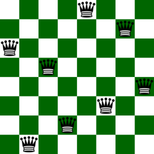
1.1.3 Modeling the 8-Queens Problem as a CSP
Given an 8x8 chessboard, place 8 queens such that no two queens threaten each other (i.e., no two queens share the same row, column, or diagonal).
Variables: (each representing the column position of a queen in each row).
Domains: for each variable.
Constraints:
Row constraints: Each queen must be in a different row (inherent in the variable definition).
Column constraints: No two queens can be in the same column.
Diagonal constraints: No two queens can be on the same diagonal.
The absolute difference between the column positions of two queens must not equal the absolute difference between their row positions. This ensures that they are not on the same diagonal. for example, if queen is in row 1 and column 3 () and queen is in row 2 and column 5 (), then:
Since 2 is not equal to 1, the queens are not on the same diagonal.
1.1.4 Solving the 8-Queens Problem using python-constraint library
from constraint import Problem, AllDifferentConstraint

def solve_8_queens():
    problem = Problem()
    #Define variables and their domains
    # Variables 1-8 represent rows, values represent column positions
    problem.addVariables(range(1, 9), range(1, 9))

    #Column constraints - all queens in different columns
    problem.addConstraint(AllDifferentConstraint(), range(1, 9))

    #Diagonal constraints - no two queens on same diagonal
    for i in range(1, 9):
        for j in range(i + 1, 9):
            # qi and qj are the column positions of queens in rows i and j
            problem.addConstraint(
                lambda qi, qj, row_diff=j-i: abs(qi - qj) != row_diff,
                (i, j)
            )

    #Get solutions
    solutions = problem.getSolutions()
    return solutions
#Solve the problem
solutions = solve_8_queens()
print(f"Number of solutions found: {len(solutions)}")
for solution in solutions:
    print(solution)
Number of solutions found: 92
{1: 8, 2: 4, 3: 1, 4: 3, 7: 7, 5: 6, 6: 2, 8: 5}
{1: 8, 2: 3, 3: 1, 4: 6, 5: 2, 6: 5, 7: 7, 8: 4}
{1: 8, 2: 2, 3: 4, 6: 5, 8: 6, 4: 1, 5: 7, 7: 3}
{1: 8, 2: 2, 3: 5, 5: 1, 4: 3, 7: 4, 6: 7, 8: 6}
{1: 7, 2: 5, 5: 6, 7: 2, 3: 3, 8: 4, 4: 1, 6: 8}
{1: 7, 2: 4, 3: 2, 4: 8, 7: 3, 5: 6, 6: 1, 8: 5}
{1: 7, 2: 4, 3: 2, 4: 5, 5: 8, 7: 3, 8: 6, 6: 1}
{1: 7, 2: 3, 3: 8, 4: 2, 7: 6, 5: 5, 6: 1, 8: 4}
{1: 7, 2: 3, 3: 1, 4: 6, 6: 5, 7: 2, 5: 8, 8: 4}
{1: 7, 2: 2, 3: 4, 5: 8, 4: 1, 6: 5, 7: 3, 8: 6}
{1: 7, 2: 2, 3: 6, 5: 1, 4: 3, 8: 5, 7: 8, 6: 4}
{1: 7, 2: 1, 3: 3, 6: 4, 8: 5, 4: 8, 5: 6, 7: 2}
{1: 6, 2: 8, 3: 2, 6: 7, 4: 4, 5: 1, 7: 5, 8: 3}
{1: 6, 2: 4, 3: 7, 4: 1, 5: 3, 6: 5, 8: 8, 7: 2}
{1: 6, 2: 4, 3: 7, 4: 1, 5: 8, 8: 3, 6: 2, 7: 5}
{1: 6, 2: 4, 3: 2, 6: 7, 4: 8, 5: 5, 7: 1, 8: 3}
{1: 6, 2: 4, 3: 1, 5: 8, 4: 5, 6: 2, 7: 7, 8: 3}
{1: 6, 2: 3, 3: 5, 6: 4, 4: 7, 5: 1, 7: 2, 8: 8}
{1: 6, 2: 3, 3: 5, 6: 4, 4: 8, 5: 1, 8: 7, 7: 2}
{1: 6, 2: 3, 3: 7, 4: 4, 5: 1, 8: 5, 6: 8, 7: 2}
{1: 6, 2: 3, 3: 7, 4: 2, 5: 4, 6: 8, 7: 1, 8: 5}
{1: 6, 2: 3, 3: 7, 4: 2, 5: 8, 6: 5, 7: 1, 8: 4}
{1: 6, 2: 3, 3: 1, 4: 8, 5: 5, 6: 2, 7: 4, 8: 7}
{1: 6, 2: 3, 3: 1, 4: 8, 5: 4, 6: 2, 7: 7, 8: 5}
{1: 6, 2: 3, 3: 1, 4: 7, 7: 2, 5: 5, 6: 8, 8: 4}
{1: 6, 2: 2, 3: 7, 4: 1, 6: 5, 7: 8, 5: 3, 8: 4}
{1: 6, 2: 2, 3: 7, 4: 1, 6: 8, 7: 5, 5: 4, 8: 3}
{1: 6, 2: 1, 3: 5, 5: 8, 4: 2, 6: 3, 7: 7, 8: 4}
{1: 5, 2: 7, 3: 4, 4: 1, 5: 3, 7: 6, 6: 8, 8: 2}
{1: 5, 2: 7, 3: 2, 4: 4, 5: 8, 6: 1, 7: 3, 8: 6}
{1: 5, 2: 7, 3: 2, 4: 6, 6: 1, 5: 3, 7: 4, 8: 8}
{1: 5, 2: 7, 3: 2, 4: 6, 6: 1, 5: 3, 7: 8, 8: 4}
{1: 5, 2: 7, 3: 1, 4: 3, 5: 8, 7: 4, 8: 2, 6: 6}
{1: 5, 2: 7, 3: 1, 4: 4, 6: 8, 5: 2, 8: 3, 7: 6}
{1: 5, 2: 8, 3: 4, 4: 1, 5: 7, 6: 2, 7: 6, 8: 3}
{1: 5, 2: 8, 3: 4, 4: 1, 5: 3, 6: 6, 7: 2, 8: 7}
{1: 5, 2: 3, 3: 8, 4: 4, 6: 1, 5: 7, 7: 6, 8: 2}
{1: 5, 2: 3, 3: 1, 4: 7, 5: 2, 7: 6, 6: 8, 8: 4}
{1: 5, 2: 3, 3: 1, 4: 6, 6: 2, 5: 8, 8: 7, 7: 4}
{1: 5, 2: 2, 3: 4, 6: 3, 4: 6, 5: 8, 7: 1, 8: 7}
{1: 5, 2: 2, 3: 4, 6: 8, 5: 3, 7: 6, 8: 1, 4: 7}
{1: 5, 2: 2, 3: 8, 4: 1, 6: 7, 7: 3, 5: 4, 8: 6}
{1: 5, 2: 2, 3: 6, 4: 1, 5: 7, 6: 4, 7: 8, 8: 3}
{1: 5, 2: 1, 3: 4, 4: 6, 5: 8, 8: 3, 6: 2, 7: 7}
{1: 5, 2: 1, 3: 8, 4: 4, 5: 2, 6: 7, 7: 3, 8: 6}
{1: 5, 2: 1, 3: 8, 4: 6, 8: 4, 5: 3, 6: 7, 7: 2}
{1: 4, 2: 6, 3: 1, 4: 5, 6: 8, 5: 2, 7: 3, 8: 7}
{1: 4, 2: 6, 3: 8, 4: 2, 5: 7, 7: 3, 6: 1, 8: 5}
{1: 4, 2: 6, 3: 8, 4: 3, 6: 7, 5: 1, 8: 2, 7: 5}
{1: 4, 2: 7, 3: 5, 6: 6, 4: 3, 5: 1, 7: 8, 8: 2}
{1: 4, 2: 7, 3: 5, 6: 1, 5: 6, 7: 3, 8: 8, 4: 2}
{1: 4, 2: 7, 3: 3, 4: 8, 5: 2, 6: 5, 7: 1, 8: 6}
{1: 4, 2: 7, 3: 1, 4: 8, 6: 2, 7: 6, 5: 5, 8: 3}
{1: 4, 2: 8, 3: 5, 4: 3, 5: 1, 8: 6, 6: 7, 7: 2}
{1: 4, 2: 8, 3: 1, 4: 3, 8: 5, 5: 6, 6: 2, 7: 7}
{1: 4, 2: 8, 3: 1, 4: 5, 5: 7, 6: 2, 7: 6, 8: 3}
{1: 4, 2: 2, 3: 7, 4: 3, 6: 8, 5: 6, 7: 1, 8: 5}
{1: 4, 2: 2, 3: 7, 4: 3, 6: 8, 5: 6, 7: 5, 8: 1}
{1: 4, 2: 2, 3: 7, 4: 5, 5: 1, 6: 8, 7: 6, 8: 3}
{1: 4, 2: 2, 3: 8, 4: 6, 5: 1, 7: 5, 8: 7, 6: 3}
{1: 4, 2: 2, 3: 8, 4: 5, 6: 1, 5: 7, 8: 6, 7: 3}
{1: 4, 2: 2, 3: 5, 4: 8, 5: 6, 7: 3, 6: 1, 8: 7}
{1: 4, 2: 1, 3: 5, 4: 8, 5: 6, 6: 3, 7: 7, 8: 2}
{1: 4, 2: 1, 3: 5, 4: 8, 5: 2, 6: 7, 7: 3, 8: 6}
{1: 3, 2: 5, 3: 2, 4: 8, 5: 6, 6: 4, 8: 1, 7: 7}
{1: 3, 2: 5, 3: 2, 4: 8, 5: 1, 8: 6, 6: 7, 7: 4}
{1: 3, 2: 5, 3: 7, 6: 2, 4: 1, 5: 4, 7: 8, 8: 6}
{1: 3, 2: 5, 3: 8, 5: 1, 4: 4, 6: 7, 7: 2, 8: 6}
{1: 3, 2: 6, 3: 4, 6: 5, 4: 2, 5: 8, 7: 7, 8: 1}
{1: 3, 2: 6, 3: 4, 6: 5, 4: 1, 5: 8, 8: 2, 7: 7}
{1: 3, 2: 6, 3: 2, 4: 5, 5: 8, 8: 4, 6: 1, 7: 7}
{1: 3, 2: 6, 3: 2, 4: 7, 5: 5, 6: 1, 7: 8, 8: 4}
{1: 3, 2: 6, 3: 2, 4: 7, 5: 1, 6: 4, 7: 8, 8: 5}
{1: 3, 2: 6, 3: 8, 4: 1, 5: 4, 6: 7, 7: 5, 8: 2}
{1: 3, 2: 6, 3: 8, 4: 1, 5: 5, 6: 7, 7: 2, 8: 4}
{1: 3, 2: 6, 3: 8, 4: 2, 7: 7, 5: 4, 6: 1, 8: 5}
{1: 3, 2: 7, 3: 2, 4: 8, 6: 4, 7: 1, 5: 6, 8: 5}
{1: 3, 2: 7, 3: 2, 4: 8, 6: 1, 7: 4, 5: 5, 8: 6}
{1: 3, 2: 8, 3: 4, 5: 1, 4: 7, 6: 6, 7: 2, 8: 5}
{1: 3, 2: 1, 3: 7, 6: 2, 4: 5, 5: 8, 7: 4, 8: 6}
{1: 2, 2: 4, 5: 3, 7: 7, 3: 6, 8: 5, 4: 8, 6: 1}
{1: 2, 2: 5, 3: 7, 4: 4, 5: 1, 7: 6, 8: 3, 6: 8}
{1: 2, 2: 5, 3: 7, 4: 1, 7: 6, 5: 3, 6: 8, 8: 4}
{1: 2, 2: 6, 3: 1, 4: 7, 7: 3, 5: 4, 6: 8, 8: 5}
{1: 2, 2: 6, 3: 8, 4: 3, 6: 4, 7: 7, 5: 1, 8: 5}
{1: 2, 2: 7, 3: 5, 5: 1, 4: 8, 6: 4, 7: 6, 8: 3}
{1: 2, 2: 7, 3: 3, 5: 8, 4: 6, 8: 4, 7: 1, 6: 5}
{1: 2, 2: 8, 3: 6, 6: 5, 8: 4, 4: 1, 5: 3, 7: 7}
{1: 1, 2: 5, 3: 8, 4: 6, 7: 2, 5: 3, 6: 7, 8: 4}
{1: 1, 2: 6, 3: 8, 4: 3, 5: 7, 6: 4, 7: 2, 8: 5}
{1: 1, 2: 7, 3: 5, 6: 4, 8: 3, 4: 8, 5: 2, 7: 6}
{1: 1, 2: 7, 3: 4, 5: 8, 4: 6, 7: 5, 6: 2, 8: 3}
1.1.5 Modeling the traveling Salesman Problem (TSP) as a CSP
The Traveling Salesman Problem (TSP) involves finding the shortest possible route that visits a set of cities and returns to the origin city.
Given a set of cities denoted by and the distances between each pair of cities denoted by , the goal is to find tour of the cities of cost at most .
There are variables , where if the tour goes directly from city to city , and otherwise.
The constraints are:
-Each city must be entered and exited exactly once:-The total cost of the tour must not exceed :
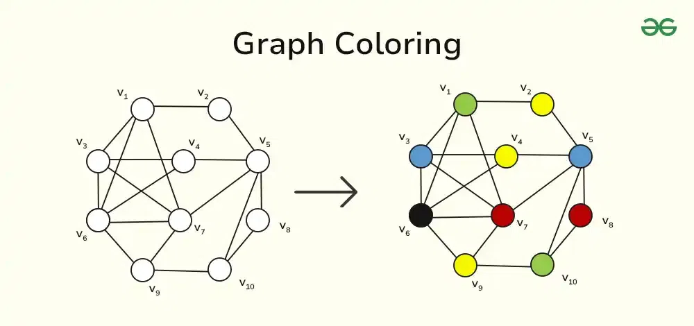
1.1.6 Modeling the graph coloring problem as a CSP
The graph coloring problem involves assigning colors to the vertices of a graph such that no two adjacent vertices share the same color.
Given an undirected graph and a set of colors , the goal is to assign a color to each vertex such that no two adjacent vertices share the same color.
This problem is closely related to the map coloring problem,wherein we wish to color the regions (e.g., provinces or states) in a map, so that each pair of adjacent regions has different colors.
The map coloring problem has practical applications in cartography, because it helps visually distinguish the different regions in the map.
Modeling the graph coloring problem as a CSP:
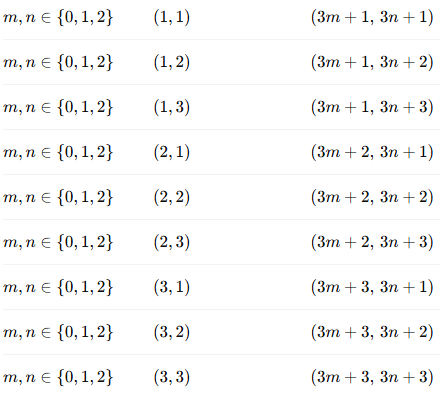
Variables: binary variables , where if vertex is assigned color , and otherwise.
Domains: for each variable.
Constraints:
Color each node exactly once:
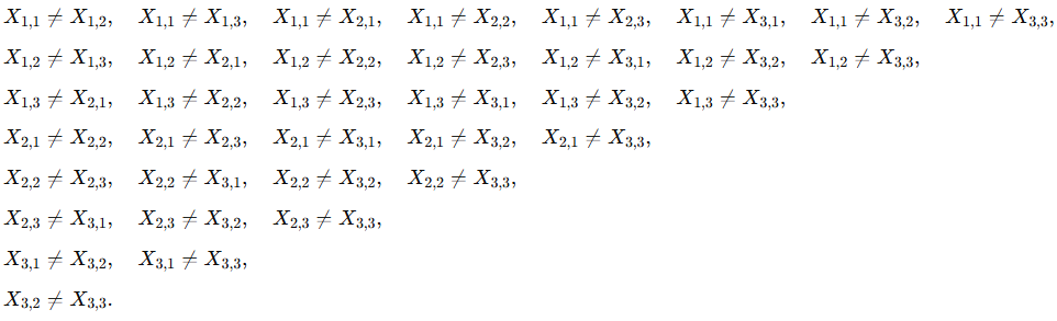
Adjacent nodes must have different colors:
1.2 Solving NP-Hard Problems
Many problems in artificial intelligence suffer from the combinatorial explosion in the number of possible solutions as the problem size increases. For example, in the case of the eight queens problem, one has to choose eight positions out of 64 positions. The number of possible solutions is given by
Generalizing the eight queens problem to the n-queens problem leads to an NP-hard setting.
The Traveling Salesman Problem (TSP) is another classic NP-hard problem where the goal is to find the shortest possible route that visits a set of cities and returns to the origin city. An instance of TSP with n cities has possible routes, which grows factorially with n.
Many other problems in AI, such as scheduling, vehicle routing, and resource allocation, are also NP-hard.
1.3 Expert Systems
Expert systems are AI programs that mimic the decision-making abilities of a human expert. They use a knowledge base of human expertise and an inference engine to solve specific problems within a certain domain.
Components of expert systems:
Knowledge Base: Contains domain-specific knowledge, including facts and rules.
Inference Engine: Applies logical rules to the knowledge base to deduce new information or make decisions.
User Interface: Allows users to interact with the expert system, input data, and receive advice or solutions.
Applications of expert systems:
Medical diagnosis (e.g., MYCIN)
Financial forecasting
Troubleshooting and repair (e.g., XCON)
For example, consider a patient, John, who comes to a doctor, while presenting the following facts about their situation:
John is running a temperature
John is coughing
John has colored phlegm
Now imagine a case where the expert system contains the following subset of rules:
IF coughing AND temperature THEN infection
IF colored phlegm AND infection THEN bacterial infection
IF bacterial infection THEN administer antibiotic
A doctor can then enter John’s symptoms in the expert system and then use a chain of inferences in order to conclude that an antibiotic needs to be administered to John.
2 Inductive Learning in Artificial Intelligence
Inductive learning involves discovering patterns from data. There are three main types:
2.1 Supervised Learning
Supervised learning learns from labeled examples to predict outputs for new inputs.
Key Idea: Given training data with known answers (labels), learn a function that maps inputs to outputs.
Mathematical Formulation:
Training data:
Goal: Learn function such that
Minimize loss:
Types of Supervised Learning:
Classification: Predict categorical labels
Binary: spam/not spam, disease/healthy
Multi-class: digit recognition (0-9), animal species
Algorithms: Logistic regression, decision trees, SVM, neural networks
Regression: Predict numerical values
Linear regression: house prices, temperature
Polynomial regression: non-linear relationships
Algorithms: Linear regression, polynomial regression, neural networks
Linear Regression Example (Conceptual):
Goal: Find line that best fits training data
Training data: (1, 3), (2, 5), (3, 7), (4, 9)

Method: Minimize sum of squared errors
  Error = Σ(actual_y - predicted_y)²

Result: y = 2x + 1

Prediction: For x=5, predict y = 2(5) + 1 = 11Analogy: Learning with a teacher who provides correct answers
2.2 Unsupervised Learning
Unsupervised learning discovers patterns in data without labeled examples.
Key Idea: Find hidden structure in unlabeled data.
Common Tasks:
Clustering: Group similar data points
K-means: Partition into k clusters
Hierarchical: Build tree of clusters
DBSCAN: Density-based clustering
Applications: Customer segmentation, document organization
Dimensionality Reduction: Compress data to fewer dimensions
PCA: Principal Component Analysis
t-SNE: Visualizing high-dimensional data
Applications: Feature extraction, data visualization
Anomaly Detection: Find unusual patterns
Isolation Forest
One-class SVM
Applications: Fraud detection, network intrusion
K-Means Clustering (Conceptual):
Algorithm: K-Means(data, k)
  1. Initialize k random centroids
  2. Repeat until convergence:
     a. Assign each point to nearest centroid
     b. Update centroids to mean of assigned points
  3. Return cluster assignments
Example:
Data: Customer purchase patterns
  - Age, annual spending

Result: 3 clusters discovered
  - Cluster 1: Young, low spending
  - Cluster 2: Middle-aged, high spending
- Cluster 3: Senior, medium spendingAnalogy: Learning without a teacher - discovering patterns on your own
2.3 Reinforcement Learning
Reinforcement learning learns by trial and error through interaction with an environment, receiving rewards or penalties.
Key Idea: An agent learns which actions to take by trying them and observing the results.
Core Components:
Agent: The learner/decision maker
Environment: What the agent interacts with
State (s): Current situation
Action (a): What the agent can do
Reward (r): Feedback (positive or negative)
Policy (\pi(s)): Strategy for selecting actions
Goal: Maximize cumulative reward over time
where (\gamma \in [0,1]) is the discount factor.
Key Algorithms:
Value-Based: Learn value function
Q-Learning
Deep Q-Networks (DQN)
Policy-Based: Learn policy directly
Policy Gradient
Actor-Critic
Model-Based: Learn environment model
AlphaZero (combines with tree search)
Multi-Armed Bandit (Simple RL Example):
Problem: Choose between k slot machines
  - Each machine has unknown reward distribution
  - Goal: Maximize total reward

Epsilon-Greedy Strategy:
  - With probability ε: explore (random action)
  - With probability 1-ε: exploit (best known action)

Example: 3 machines with true values [1.0, 2.0, 1.5]
  After 1000 trials:
    Learned estimates: [0.98, 2.02, 1.47]
    Machine 2 selected 70% of the time
Applications:
Game playing: AlphaGo, AlphaZero, OpenAI Five
Robotics: Walking, manipulation, navigation
Autonomous vehicles: Decision making
Resource management: Data center cooling, traffic lights
Analogy: Like training a dog - reward good behavior, penalize bad behavior
Comparing Learning Types
| Aspect | Supervised | Unsupervised | Reinforcement |
|---|---|---|---|
| Data | Labeled examples | Unlabeled data | Interaction with environment |
| Feedback | Correct answers | None (implicit structure) | Rewards/penalties |
| Goal | Predict outputs | Discover patterns | Maximize cumulative reward |
| Training | (X, y) pairs | X only | (s, a, r, s’) tuples |
| Example | Spam detection | Customer segmentation | Game playing |
| Learning | From examples | From structure | From experience |
| Evaluation | Accuracy on test set | Cluster quality | Total reward earned |